Partitional and Hierarchical Based clustering Lecture 22 Based
Partitional and Hierarchical Based clustering Lecture 22 Based on Slides of Dr. Ikle & chapter 8 of Tan, Steinbach, Kumar
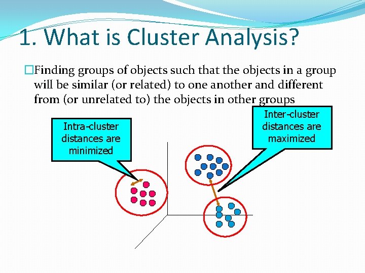
1. What is Cluster Analysis? �Finding groups of objects such that the objects in a group will be similar (or related) to one another and different from (or unrelated to) the objects in other groups Intra-cluster distances are minimized Inter-cluster distances are maximized
Examples of Clustering • • • Biology: kingdom, phylum, class, order, family, genus, and species Information Retrieval: search engine query = movie, clusters = reviews, trailers, stars, theaters Climate: Clusters = regions of similar climate Psychology and Medicine: patterns in spatial or temporal distribution of a disease Business: Segment customers into groups for marketing activities
Two Reasons for Clustering • • Clustering for Understanding • (see examples from previous slide) Clustering for Utility • Summarizing: different algorithms can run faster on a data set summarized by clustering • Compression: storing cluster information is more efficient that storing the entire data - example: quantization • Finding Nearest Neighbors
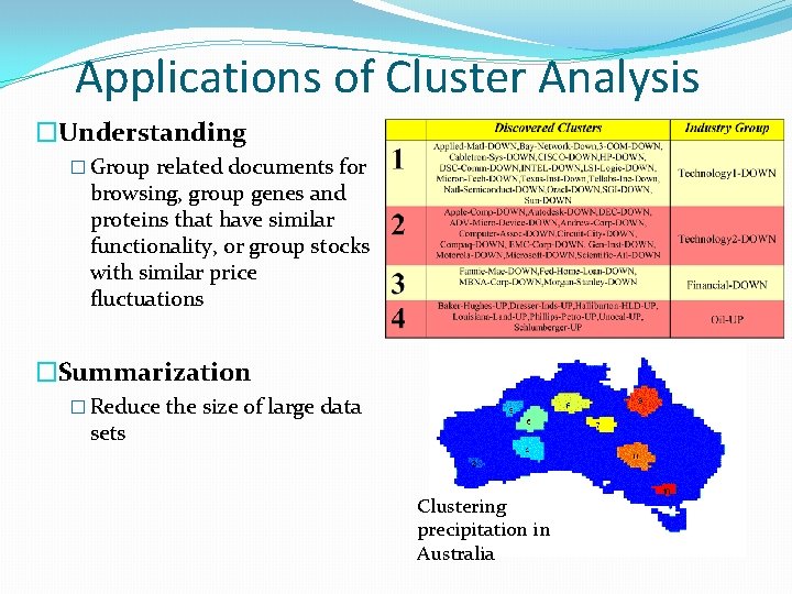
Applications of Cluster Analysis �Understanding � Group related documents for browsing, group genes and proteins that have similar functionality, or group stocks with similar price fluctuations �Summarization � Reduce the size of large data sets Clustering precipitation in Australia
CLUSTERING: Introduction �Clustering �No class to be predicted �Groups objects based solely on their attributes �Objects within clusters similar to each other �Objects in different clusters dissimilar to each other �Depends on similarity measure �Clustering as unsupervised classification
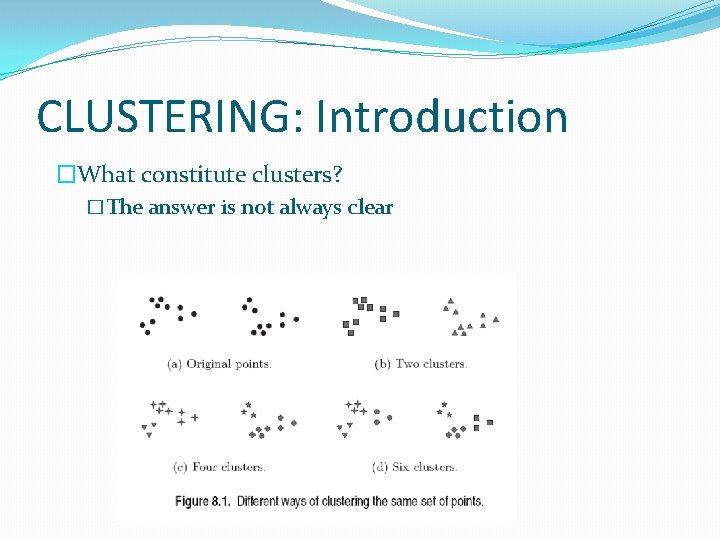
CLUSTERING: Introduction �What constitute clusters? �The answer is not always clear
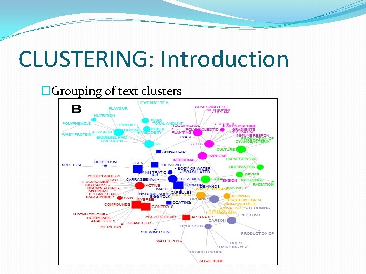
CLUSTERING: Introduction �Grouping of text clusters
CLUSTERING: Introduction �Types of clustering �Partitional � Simple division of instances into mutually exclusive (non-overlapping) clusters � Determine desired number of clusters � Iteratively reallocate objects to clusters
1: Introduction �Types of clustering �Hierarchical � Clusters allowed to have (nested) subclusters � Uses previous clusters to find subclusters � Types of hierarchical algorithms �Agglomerative (bottom-up) �Merge smaller clusters �Divisive (top-down) �Divide larger clusters
CLUSTERING: Common Algorithms �Partitional �K-means �K-medoids �Density-based �DBSCAN �SNN
2. K-Means Clustering • • K-means clustering is one of the most common/popular techniques Each cluster is associated with a centroid (center point) – this is often the mean – it is the cluster prototype Each point is assigned to the cluster with the closest centroid The number of clusters, K, must be specified ahead of time
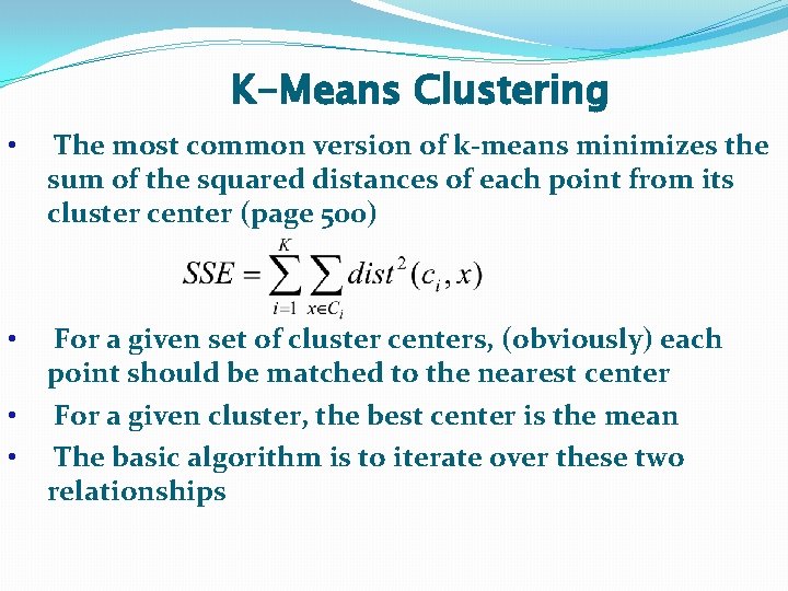
K-Means Clustering • The most common version of k-means minimizes the sum of the squared distances of each point from its cluster center (page 500) • For a given set of cluster centers, (obviously) each point should be matched to the nearest center For a given cluster, the best center is the mean The basic algorithm is to iterate over these two relationships • •
2. CLUSTERING: K-means �Pseudo-code �Choose number of clusters, k �Initialize k centroids (randomly, for example) �Repeat � Form k clusters by assigning each point to its nearest centroid � Recalculate centroids �Until convergence (centroids move less than some amount)
CLUSTERING: K-means �Time complexity �O(n*k*l*d) � n=number of points � k=number of clusters � l=number of iterations � d=number of attributes �Space complexity �O(k+n)
CLUSTERING: K-means �Time complexity �O(n*k*l*d) � n=number of points � k=number of clusters � l=number of iterations � d=number of attributes �Space complexity �O(k+n)
K-means disadvantages �Bad choice for k may yield poor results �Fixed number of clusters makes it difficult to determine best value for k �Dependent upon choice of initial centroids �Really only works well for “spherical” cluster shapes
CLUSTERING: K-means advantages �Simple and effective �Conceptually �To implement �To run �Other algorithms require more parameters to adjust �Relatively quick
CLUSTERING: K-means solutions �One does not always need high quality clusters �Can use multiple runs to help with initial centroids �Choose best final result �Probability is not your friend �Run with different values for k and obtain the best result �Produce hierarchical clustering �Set k=2 �Repeat recursively within each cluster

CLUSTERING: K-means solutions �One does not always need high quality clusters �Can use multiple runs to help with initial centroids �Choose best final result �Probability is not your friend �Run with different values for k and obtain the best result �Produce hierarchical clustering �Set k=2 �Repeat recursively within each cluster
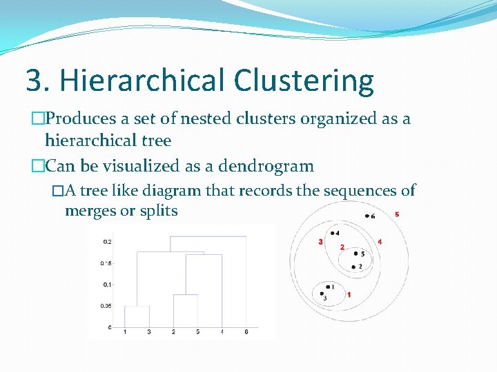
3. Hierarchical Clustering �Produces a set of nested clusters organized as a hierarchical tree �Can be visualized as a dendrogram �A tree like diagram that records the sequences of merges or splits
Strengths of Hierarchical Clustering �Do not have to assume any particular number of clusters �Any desired number of clusters can be obtained by ‘cutting’ the dendogram at the proper level �They may correspond to meaningful taxonomies �Example in biological sciences (e. g. , animal kingdom, phylogeny reconstruction, …)
Hierarchical Clustering �Two main types of hierarchical clustering � Agglomerative: � Start with the points as individual clusters � At each step, merge the closest pair of clusters until only one cluster (or k clusters) left � Divisive: � Start with one, all-inclusive cluster � At each step, split a cluster until each cluster contains a point (or there are k clusters) �Traditional hierarchical algorithms use a similarity or distance matrix � Merge or split one cluster at a time
Agglomerative Clustering Algorithm � More popular hierarchical clustering technique � Basic algorithm is straightforward 1. 2. 3. 4. 5. 6. Compute the proximity matrix Let each data point be a cluster Repeat Merge the two closest clusters Update the proximity matrix Until only a single cluster remains � Key operation is the computation of the proximity of two clusters � Different approaches to defining the distance between clusters distinguish the different algorithms
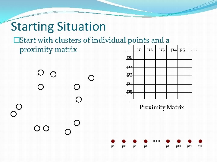
Starting Situation �Start with clusters of individual points and a p 1 p 2 p 3 p 4 proximity matrix p 5 p 1 p 2 p 3 p 4 p 5. . . Proximity Matrix . . .
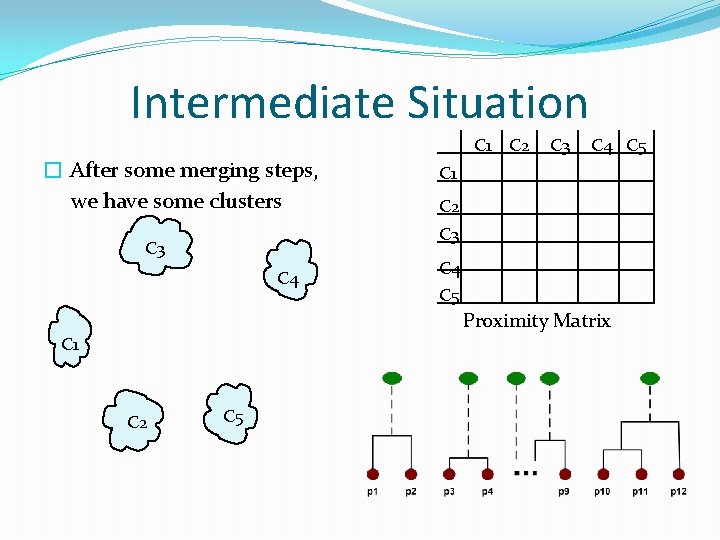
Intermediate Situation � After some merging steps, we have some clusters C 1 C 2 C 3 C 4 C 5 Proximity Matrix C 1 C 2 C 5
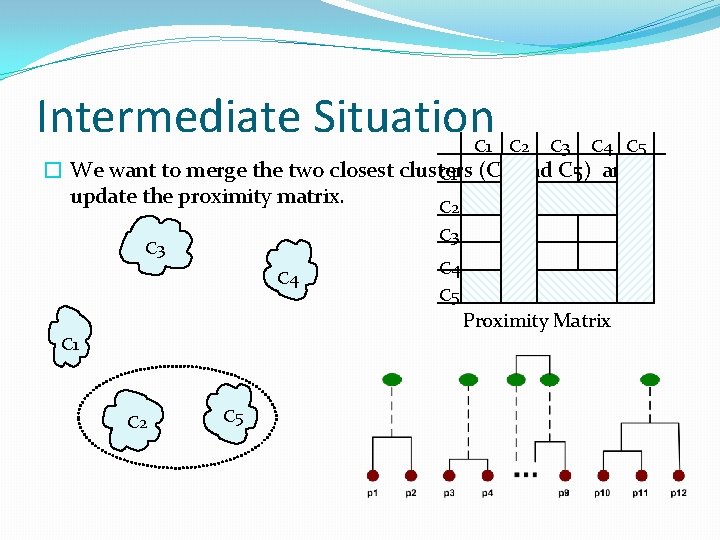
Intermediate Situation C 1 C 2 C 3 C 4 C 5 � We want to merge the two closest clusters C 1 (C 2 and C 5) and update the proximity matrix. C 2 C 3 C 4 C 5 Proximity Matrix C 1 C 2 C 5
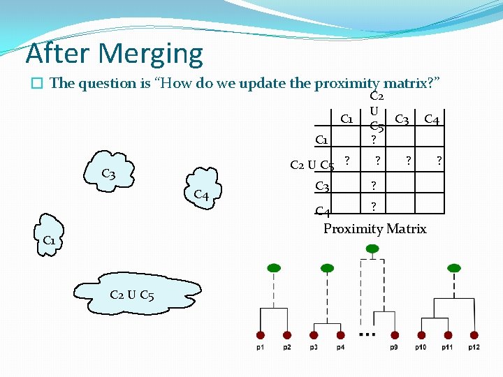
After Merging � The question is “How do we update the proximity matrix? ” C 1 C 2 U C 5 ? C 3 C 4 C 2 U C 3 C 5 ? ? C 3 ? C 4 ? Proximity Matrix C 1 C 2 U C 5 ?
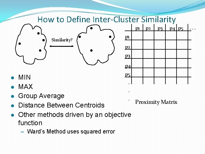
How to Define Inter-Cluster Similarity p 1 Similarity? p 2 p 3 p 4 p 5 p 1 p 2 p 3 p 4 l l l p 5 MIN. MAX. Group Average. Proximity Matrix Distance Between Centroids Other methods driven by an objective function – Ward’s Method uses squared error . . .
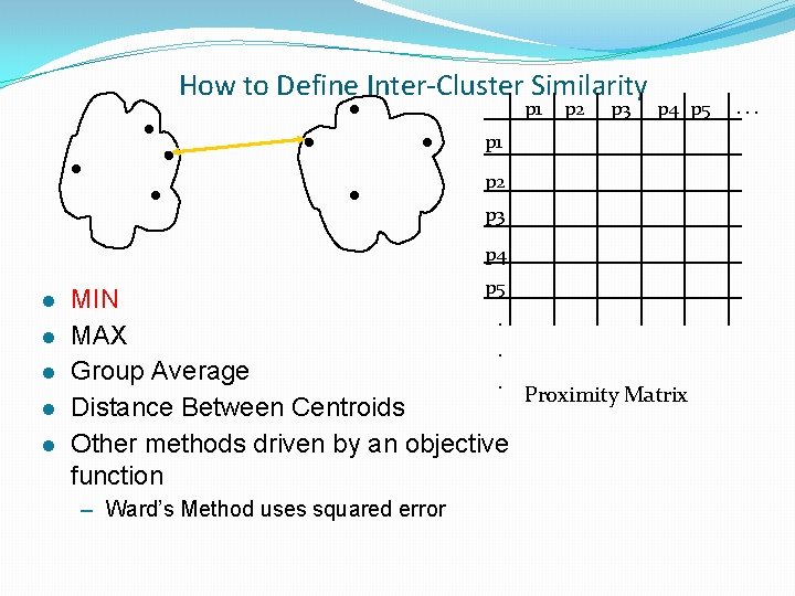
How to Define Inter-Cluster Similarity p 1 p 2 p 3 p 4 p 5 p 1 p 2 p 3 p 4 l l l p 5 MIN. MAX. Group Average. Proximity Matrix Distance Between Centroids Other methods driven by an objective function – Ward’s Method uses squared error . . .
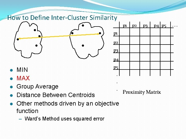
How to Define Inter-Cluster Similarity p 1 p 2 p 3 p 4 p 5 p 1 p 2 p 3 p 4 l l l p 5 MIN. MAX. Group Average. Proximity Matrix Distance Between Centroids Other methods driven by an objective function – Ward’s Method uses squared error . . .
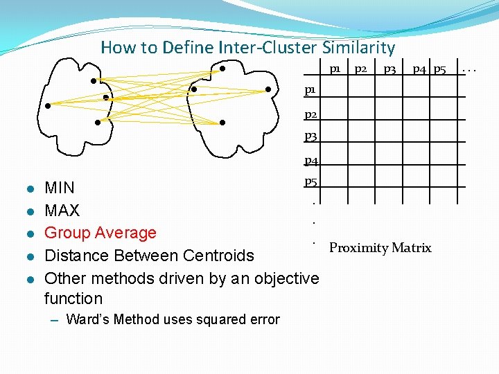
How to Define Inter-Cluster Similarity p 1 p 2 p 3 p 4 p 5 p 1 p 2 p 3 p 4 l l l p 5 MIN. MAX. Group Average. Proximity Matrix Distance Between Centroids Other methods driven by an objective function – Ward’s Method uses squared error . . .
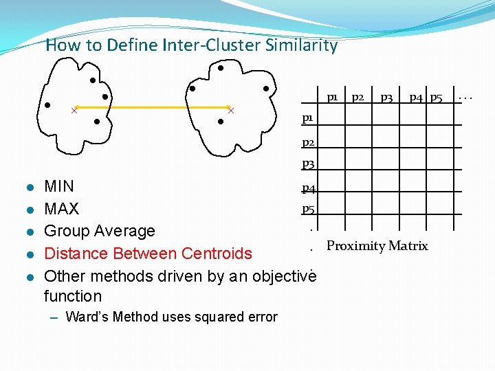
How to Define Inter-Cluster Similarity p 1 p 2 p 3 p 4 p 5 p 1 p 2 p 3 l l l p 4 MIN p 5 MAX. Group Average. Proximity Matrix Distance Between Centroids. Other methods driven by an objective function – Ward’s Method uses squared error . . .
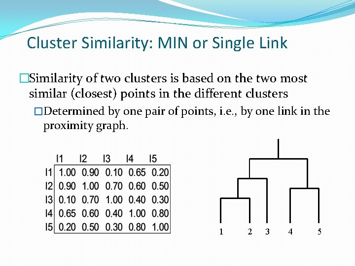
Cluster Similarity: MIN or Single Link �Similarity of two clusters is based on the two most similar (closest) points in the different clusters �Determined by one pair of points, i. e. , by one link in the proximity graph. 1 2 3 4 5
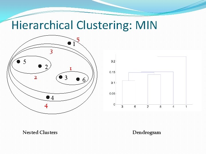
Hierarchical Clustering: MIN 1 3 5 2 1 2 3 4 5 6 4 Nested Clusters Dendrogram
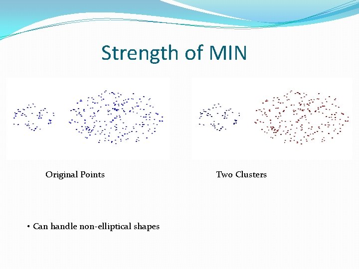
Strength of MIN Original Points • Can handle non-elliptical shapes Two Clusters
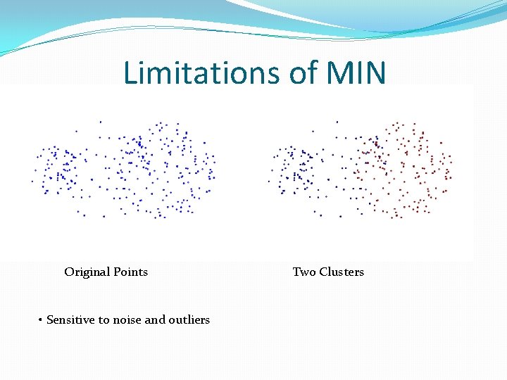
Limitations of MIN Original Points • Sensitive to noise and outliers Two Clusters
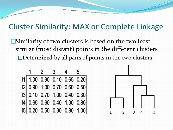
Cluster Similarity: MAX or Complete Linkage �Similarity of two clusters is based on the two least similar (most distant) points in the different clusters �Determined by all pairs of points in the two clusters 1 2 3 4 5
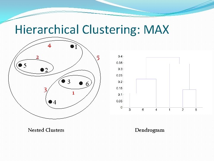
Hierarchical Clustering: MAX 4 1 5 2 3 3 6 1 4 Nested Clusters Dendrogram
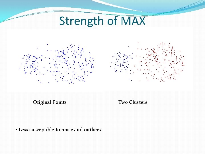
Strength of MAX Original Points • Less susceptible to noise and outliers Two Clusters
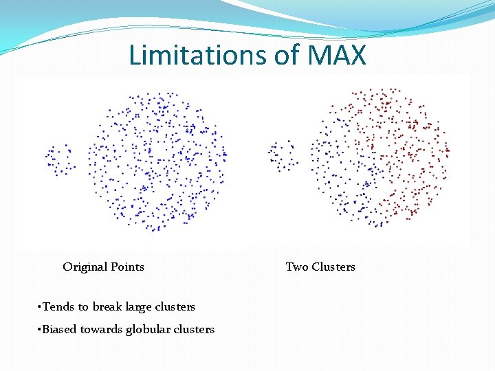
Limitations of MAX Original Points • Tends to break large clusters • Biased towards globular clusters Two Clusters
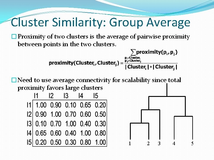
Cluster Similarity: Group Average �Proximity of two clusters is the average of pairwise proximity between points in the two clusters. �Need to use average connectivity for scalability since total proximity favors large clusters 1 2 3 4 5
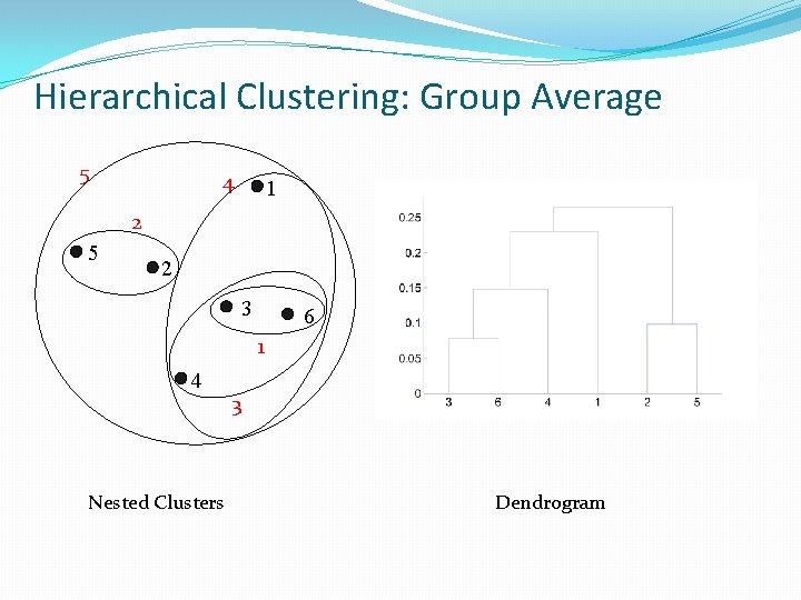
Hierarchical Clustering: Group Average 5 4 1 2 5 2 3 6 1 4 Nested Clusters 3 Dendrogram
Hierarchical Clustering: Group Average � Compromise between Single and Complete Link � Strengths � Less susceptible to noise and outliers � Limitations � Biased towards globular clusters
Cluster Similarity: Ward’s Method �Similarity of two clusters is based on the increase in squared error when two clusters are merged �Similar to group average if distance between points is distance squared �Less susceptible to noise and outliers �Biased towards globular clusters �Hierarchical analogue of K-means �Can be used to initialize K-means
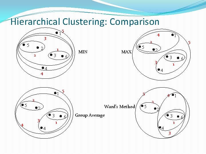
Hierarchical Clustering: Comparison 1 3 5 5 4 1 3 4 6 MIN MAX 5 5 1 5 Ward’s Method 3 6 5 4 1 2 2 Group Average 3 1 4 6 4 2 3 3 3 2 4 1 5 5 2 2 2 1 1 4 3 6
Hierarchical Clustering: Time and Space requirements �O(N 2) space since it uses the proximity matrix. �N is the number of points. �O(N 3) time in many cases �There are N steps and at each step the size, N 2, proximity matrix must be updated and searched �Complexity can be reduced to O(N 2 log(N) ) time for some approaches
Hierarchical Clustering: Problems and Limitations �Once a decision is made to combine two clusters, it cannot be undone �No objective function is directly minimized �Different schemes have problems with one or more of the following: �Sensitivity to noise and outliers �Difficulty handling different sized clusters and convex shapes �Breaking large clusters
- Slides: 48