Partition Based Spatial Merge Join Present by Tony

Partition Based Spatial – Merge Join Present by: Tony Tong (09049620) Cleo Tsang (09049630) June Yau (09030360) Chelsie Chan (10104740) Oengus Lam (10104790) 1

Agenda 1. 2. 3. 4. 5. Problem Definition of Spatial Join PBSM Algorithm 3. 1 Filter Step 3. 2 Refinement Step 3. 3 Number of Partition 3. 4 Spatial Partitioning Function Performance 4. 1 Indexed Nested Loops Join 4. 2 R-tree Based Join Algorithm 4. 3 Methodology 4. 4 None of Indices Pre-exist 4. 5 In the Presence of Pre-existing Index 4. 6 CPU Costs Conclusion 2

1. Problem • In a spatial database system, like GIS, join queries objects involve large amount of memory • Have no pre computing data for datasets • Usually no index for intermediate result • Solve this join problem efficiently 3

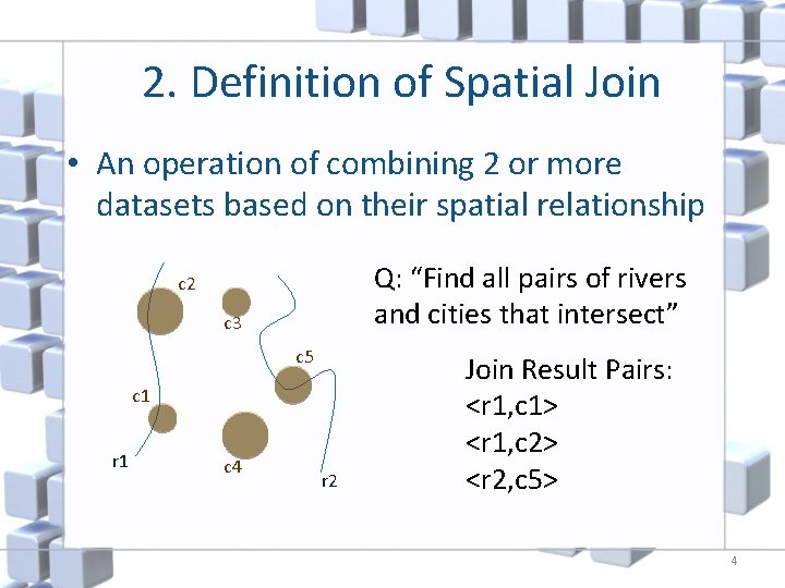
2. Definition of Spatial Join • An operation of combining 2 or more datasets based on their spatial relationship Q: “Find all pairs of rivers and cities that intersect” c 2 c 3 c 5 c 1 r 1 c 4 r 2 Join Result Pairs: <r 1, c 1> <r 1, c 2> <r 2, c 5> 4

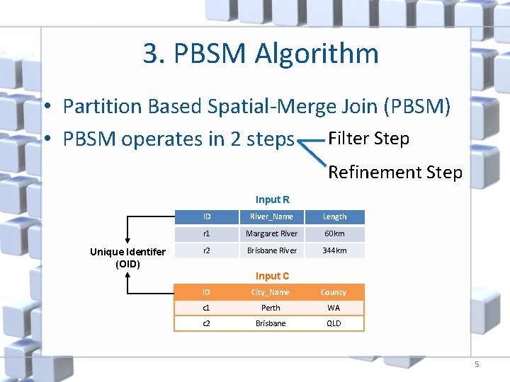
3. PBSM Algorithm • Partition Based Spatial-Merge Join (PBSM) • PBSM operates in 2 steps Filter Step Refinement Step Input R Unique Identifer (OID) ID River_Name Length r 1 Margaret River 60 km r 2 Brisbane River 344 km Input C ID City_Name County c 1 Perth WA c 2 Brisbane QLD 5

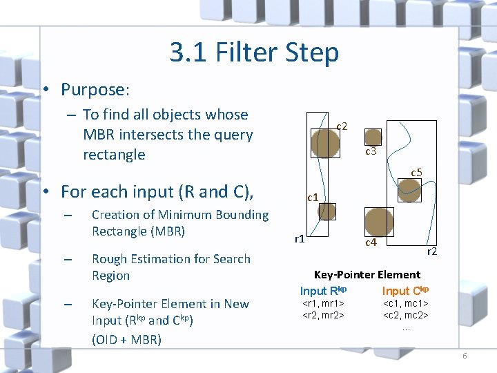
3. 1 Filter Step • Purpose: – To find all objects whose MBR intersects the query rectangle c 2 c 3 c 5 • For each input (R and C), – – – Creation of Minimum Bounding Rectangle (MBR) Rough Estimation for Search Region Key-Pointer Element in New Input (Rkp and Ckp) (OID + MBR) c 1 r 1 c 4 r 2 Key-Pointer Element Input Rkp Input Ckp <r 1, mr 1> <r 2, mr 2> <c 1, mc 1> <c 2, mc 2>. . . 6

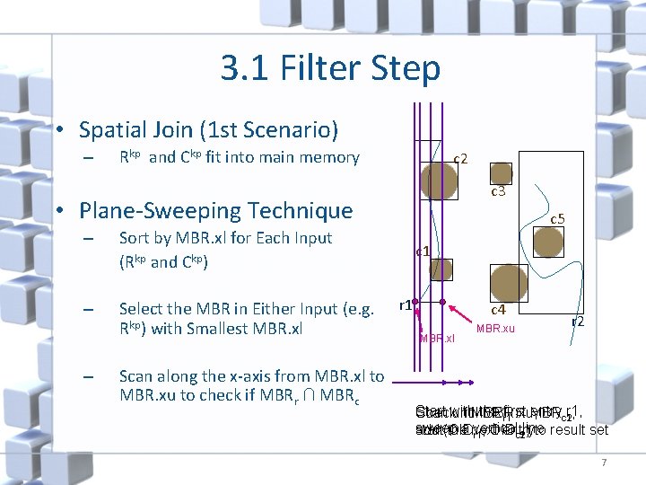
3. 1 Filter Step • Spatial Join (1 st Scenario) – Rkp and Ckp fit into main memory c 2 c 3 • Plane-Sweeping Technique – Sort by MBR. xl for Each Input (Rkp and Ckp) – Select the MBR in Either Input (e. g. Rkp) with Smallest MBR. xl – Scan along the x-axis from MBR. xl to MBR. xu to check if MBRr ∩ MBRc c 5 c 1 r 1 c 4 MBR. xl MBR. xu r 2 Start the first entryc 2 r 1, Checkwith if MBR , Scan until MBR. xu, r 1 ∩ MBRc 1 sweep vertical line add (OID start thea next entry r 1, OID c 2) to result set c 1 7

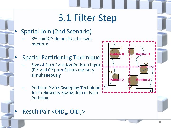
3. 1 Filter Step • Spatial Join (2 nd Scenario) – Rkp and Ckp do not fit into main memory • Spatial Partitioning Technique – Size of Each Partition for both Input (Rkp and Ckp) can fit into memory simultaneously c 2 Partition 0 c 3 c 5 c 1 Partition 3 Partition 2 – Perform Plane-Sweeping Technique r 1 for Preliminary Spatial Join in Each Partition 1 c 4 r 2 • Result Pair <OIDR, OIDC> 8

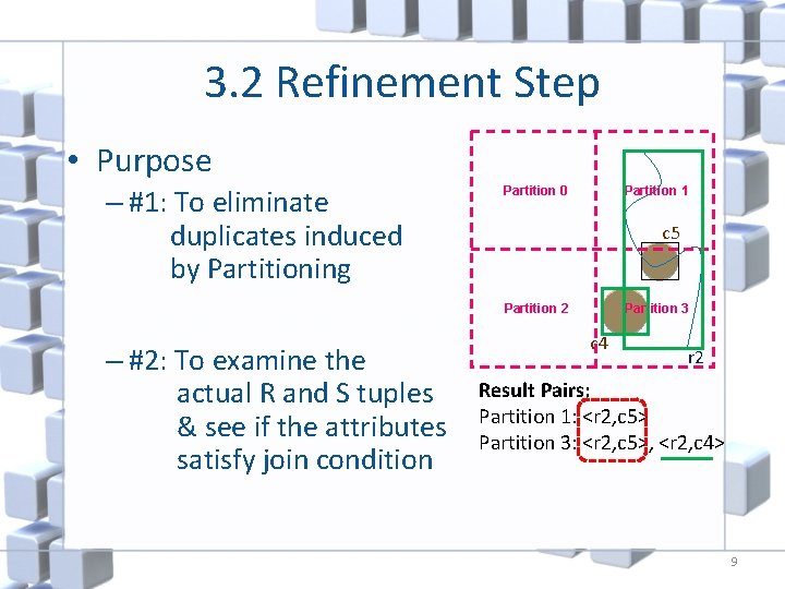
3. 2 Refinement Step • Purpose – #1: To eliminate duplicates induced by Partitioning Partition 1 Partition 0 c 5 Partition 3 Partition 2 – #2: To examine the actual R and S tuples & see if the attributes satisfy join condition c 4 r 2 Result Pairs: Partition 1: <r 2, c 5> Partition 3: <r 2, c 5>, <r 2, c 4> 9

3. 2 Refinement Step • Procedure – #1: Sort OID pairs: • Primary Sort Key: OIDR • Secondary Sort Key: OIDC – #2: Read R tuples first, then C

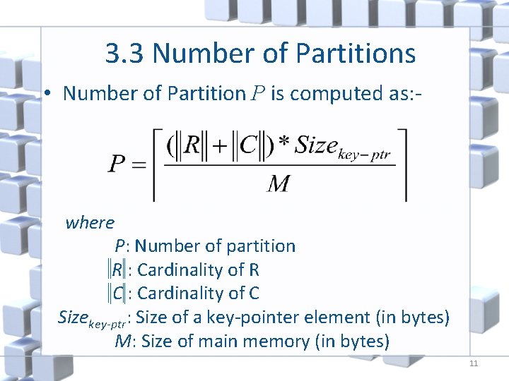
3. 3 Number of Partitions • Number of Partition P is computed as: - where P: Number of partition R : Cardinality of R C : Cardinality of C Sizekey-ptr: Size of a key-pointer element (in bytes) M: Size of main memory (in bytes) 11

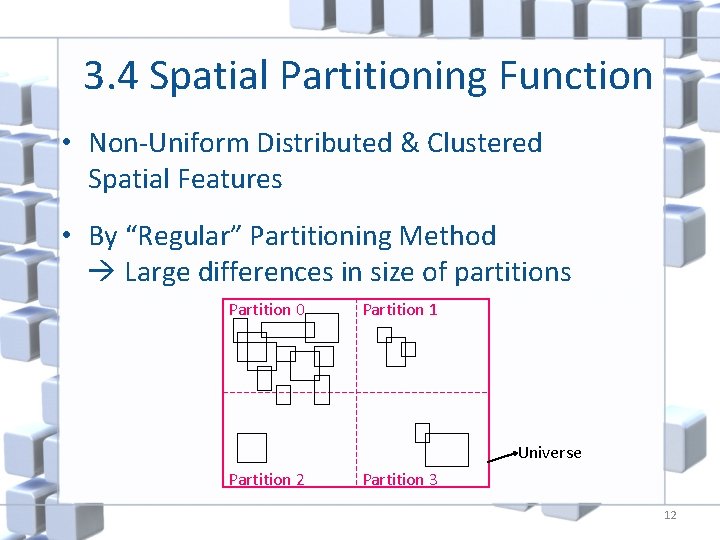
3. 4 Spatial Partitioning Function • Non-Uniform Distributed & Clustered Spatial Features • By “Regular” Partitioning Method Large differences in size of partitions Partition 0 Partition 1 Universe Partition 2 Partition 3 12

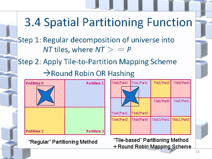
3. 4 Spatial Partitioning Function Step 1: Regular decomposition of universe into NT tiles, where NT ＞ ＝ P Step 2: Apply Tile-to-Partition Mapping Scheme Round Robin OR Hashing Partition 0 Partition 2 Partition 1 Tile 0/Part 0 Tile 1/Part 1 Tile 4/Part 1 Tile 5/Part 2 Tile 8/Part 2 Tile 9/Part 0 Tile 2/Part 2 Tile 3/Part 0 Tile 6/Part 0 Tile 7/Part 1 Tile 10/Part 1 Tile 11/Part 2 Partition 3 “Regular” Partitioning Method “Tile-based” Partitioning Method + Round Robin Mapping Scheme 13

3. 4 Spatial Partitioning Function • What is the PERFECT Spatial Partitioning Function ? • Considerations: It assigns equal number of tuples to each partition – Number of Tiles – Tile-to-Partition Mapping Scheme (Round Robin OR Hashing) • Data set used for investigation: – Tiger Road Data (62. 4 MB, 456, 613 tuples) – Sequoia Polygon Data (21. 9 MB, 58, 115 tuples) 14

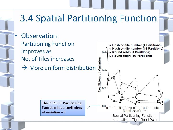
3. 4 Spatial Partitioning Function • Observation: Partitioning Function improves as No. of Tiles increases More uniform distribution The PERFECT Partitioning Function has a coefficient of variation = 0 Spatial Partitioning Function Alternatives: Tiger Road Data 15

3. 4 Spatial Partitioning Function • Observation: ↑ No. of Tiles, ↑ Replication Overhead Number of Tiles = An integral multiple of Number of Partitions Replication Overhead: Tiger Road Data (16 Partitions) Replication Overhead: Sequoia Polygon Data(16 Partitions) 16

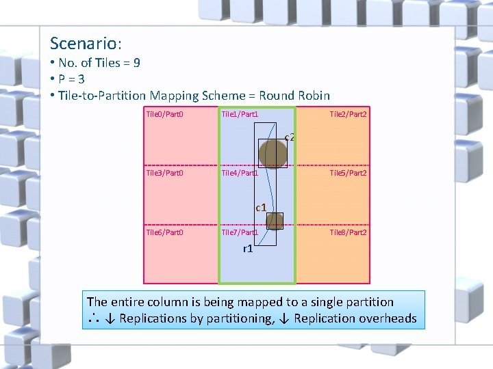
Scenario: • No. of Tiles = 9 • P=3 • Tile-to-Partition Mapping Scheme = Round Robin Tile 0/Part 0 Tile 1/Part 1 Tile 2/Part 2 c 2 Tile 3/Part 0 Tile 4/Part 1 Tile 5/Part 2 c 1 Tile 6/Part 0 Tile 7/Part 1 Tile 8/Part 2 r 1 The entire column is being mapped to a single partition ∴ ↓ Replications by partitioning, ↓ Replication overheads

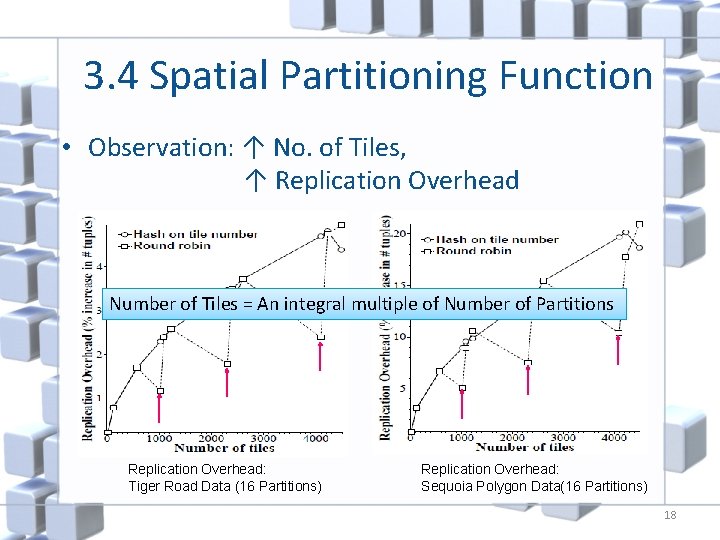
3. 4 Spatial Partitioning Function • Observation: ↑ No. of Tiles, ↑ Replication Overhead Number of Tiles = An integral multiple of Number of Partitions Replication Overhead: Tiger Road Data (16 Partitions) Replication Overhead: Sequoia Polygon Data(16 Partitions) 18

4. Performance Indexed Nested Loops Join V. S PBSM Join (1024 tiles) V. S R-tree Based Join 19

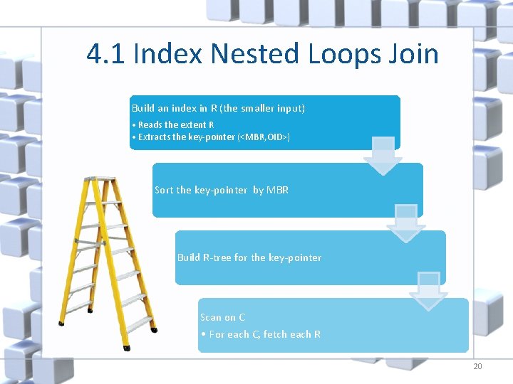
4. 1 Index Nested Loops Join Build an index in R (the smaller input) • Reads the extent R • Extracts the key-pointer (<MBR, OID>) Sort the key-pointer by MBR Build R-tree for the key-pointer Scan on C • For each C, fetch each R 20

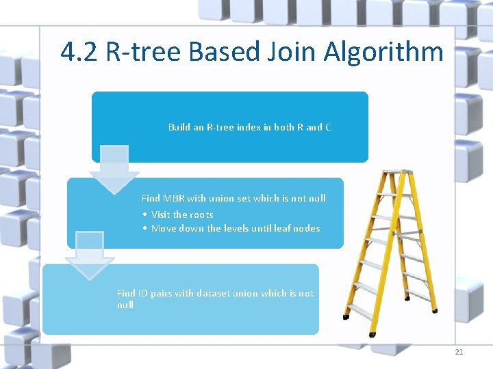
4. 2 R-tree Based Join Algorithm Build an R-tree index in both R and C Find MBR with union set which is not null • Visit the roots • Move down the levels until leaf nodes Find ID pairs with dataset union which is not null 21

4. 3 Methodology • Database System: Paradise • Machine: Sun SPARC-10/51 – 64 MB of memory – Sun. OS Release 4. 1. 3 – One Seagate 2 GB disk 22

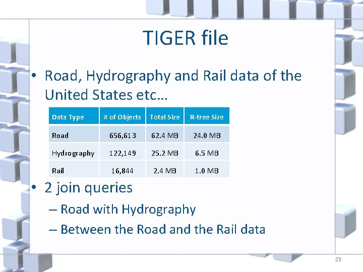
TIGER file • Road, Hydrography and Rail data of the United States etc… Data Type # of Objects Total Size R-tree Size Road 656, 613 62. 4 MB 24. 0 MB Hydrography 122, 149 25. 2 MB 6. 5 MB Rail 16, 844 2. 4 MB 1. 0 MB • 2 join queries – Road with Hydrography – Between the Road and the Rail data 23

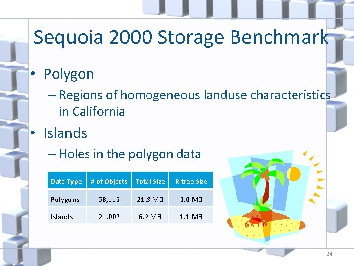
Sequoia 2000 Storage Benchmark • Polygon – Regions of homogeneous landuse characteristics in California • Islands – Holes in the polygon data Data Type # of Objects Total Size R-tree Size Polygons 58, 115 21. 9 MB 3. 0 MB Islands 21, 007 6. 2 MB 1. 1 MB 24

4. 4 NONE OF INDICES PRE-EXIST 25

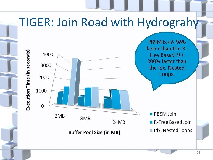
TIGER: Join Road with Hydrograhy PBSM is 48 -98% faster than the RTree Based; 93300% faster than the Idx. Nested Loops. 26

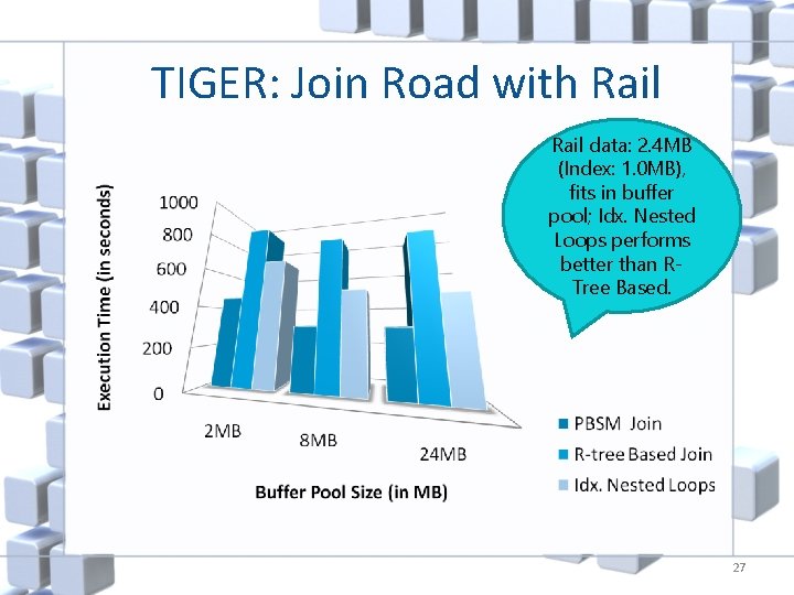
TIGER: Join Road with Rail data: 2. 4 MB (Index: 1. 0 MB), fits in buffer pool; Idx. Nested Loops performs better than RTree Based. 27

Cluster • Data continuously , i. e. not randomly distributed • Data are mostly in sequential order in real life • Less computationally expensive 28

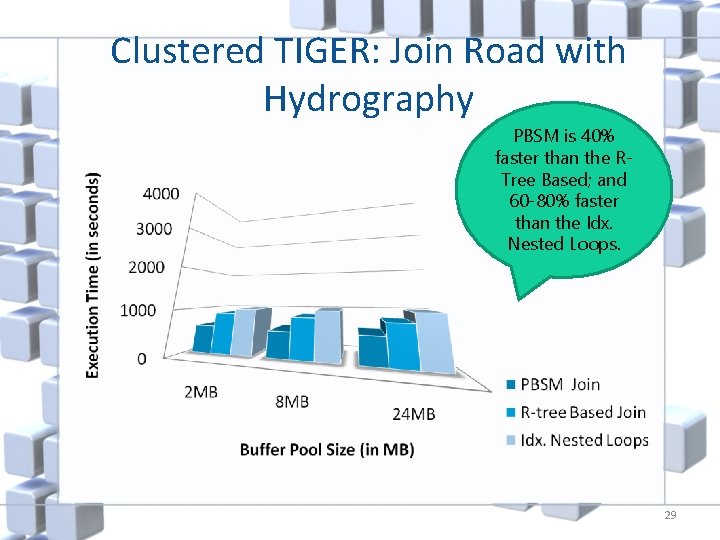
Clustered TIGER: Join Road with Hydrography PBSM is 40% faster than the RTree Based; and 60 -80% faster than the Idx. Nested Loops. 29

Costs • Index Building Cost – Cost of extracting the key-pointers from the input – Sorting the key-pointers – Building the index using the sorted key pointers – If Input is clustered No sorting key-pointers Cost of building index • Tree Joining Cost • Refinement Step Cost 30

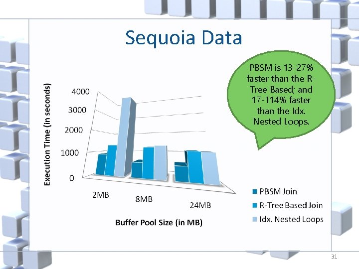
Sequoia Data PBSM is 13 -27% faster than the RTree Based; and 17 -114% faster than the Idx. Nested Loops. 31

Summary • PBSM is better than R-tree and the Indexed Nested Loops based algorithm • When sizes of 2 inputs differ significantly, Indexed Nested Loops is better than the Rtree based algorithm • All algorithms improve if join inputs are clustered 32

4. 5 IN THE PRESENCE OF PRE -EXISTING INDEX 33

TIGER: Join Road with Hydrograhy When indices pre -exist on both the inputs, the Rtree based algorithm has the best performance 34

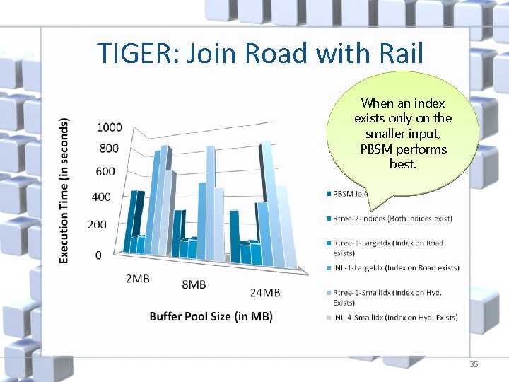
TIGER: Join Road with Rail When an index exists only on the smaller input, PBSM performs best. 35

4. 6 CPU Cost • Insert a table • CPU cost > I/O cost • System – CPU intensive – Much less I/O is needed 36

5. Principal Behind • Divide and Conquer • Optimization on memory size

6. Playback of this presentation • • • Efficient PBSM algorithm Comparison among different algorithm Performance Analysis Clustered Data Indexed Data 38

Question ? 39