Particle FilterMonte Carlo Localization Slides from D Fox

Particle Filter/Monte Carlo Localization Slides from D. Fox. W. Burgard, C. Stachniss, M. Bennewitz, K. Arras, S. Thrun, J. Xiao 1

Particle Filter Definition: ØParticle filter is a Bayesian based filter that sample the whole robot work space by a weight function derived from the belief distribution of previous stage. Basic principle: ØSet of state hypotheses (“particles”) ØSurvival-of-the-fittest 2

Why Particle Filters § Represent belief by random samples § Estimation of non-Gaussian, nonlinear processes Ø Particle filtering non-parametric inference algorithm - suited to track non-linear dynamics. - efficiently represent non-Gaussian distributions

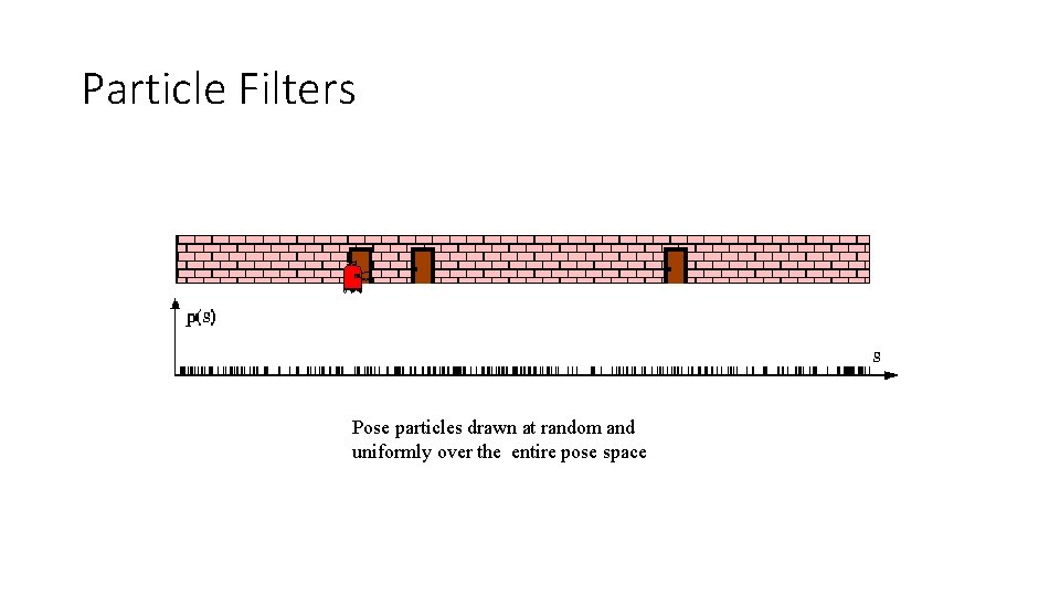
Particle Filters Pose particles drawn at random and uniformly over the entire pose space

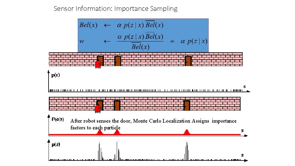
Sensor Information: Importance Sampling After robot senses the door, Monte Carlo Localization Assigns importance factors to each particle

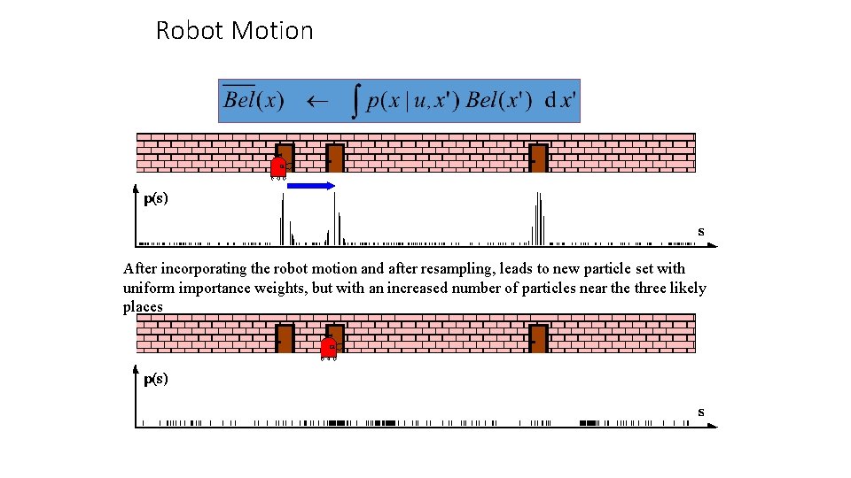
Robot Motion After incorporating the robot motion and after resampling, leads to new particle set with uniform importance weights, but with an increased number of particles near the three likely places

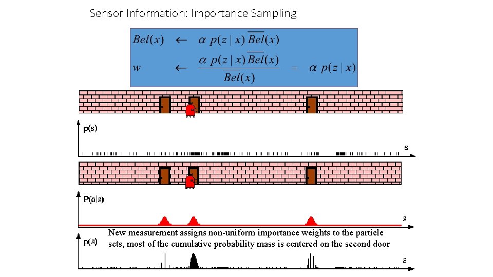
Sensor Information: Importance Sampling New measurement assigns non-uniform importance weights to the particle sets, most of the cumulative probability mass is centered on the second door

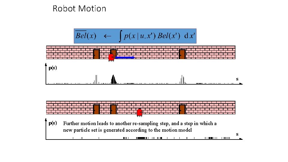
Robot Motion Further motion leads to another re-sampling step, and a step in which a new particle set is generated according to the motion model

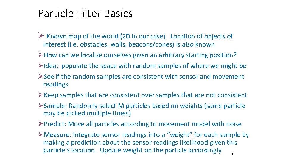
Particle Filter Basics Ø Known map of the world (2 D in our case). Location of objects of interest (i. e. obstacles, walls, beacons/cones) is also known ØHow can we localize ourselves given an arbitrary starting position? ØIdea: populate the space with random samples of where we might be ØSee if the random samples are consistent with sensor and movement readings ØKeep samples that are consistent over samples that are not consistent ØSample: Randomly select M particles based on weights (same particle may be picked multiple times) ØPredict: Move all particles according to movement model with noise ØMeasure: Integrate sensor readings into a “weight” for each sample by making a prediction about the sensor readings likelihood given this particle’s location. Update weight on the particle accordingly 9

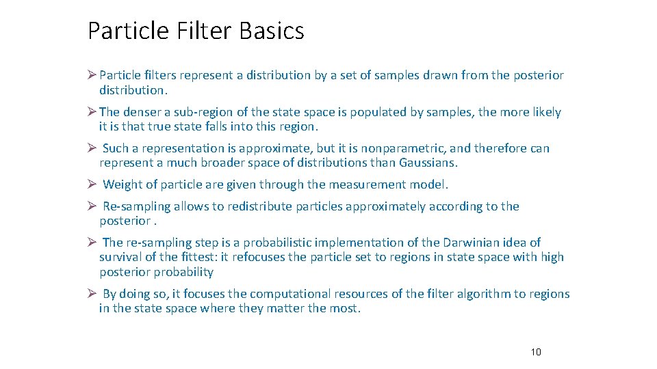
Particle Filter Basics Ø Particle filters represent a distribution by a set of samples drawn from the posterior distribution. Ø The denser a sub-region of the state space is populated by samples, the more likely it is that true state falls into this region. Ø Such a representation is approximate, but it is nonparametric, and therefore can represent a much broader space of distributions than Gaussians. Ø Weight of particle are given through the measurement model. Ø Re-sampling allows to redistribute particles approximately according to the posterior. Ø The re-sampling step is a probabilistic implementation of the Darwinian idea of survival of the fittest: it refocuses the particle set to regions in state space with high posterior probability Ø By doing so, it focuses the computational resources of the filter algorithm to regions in the state space where they matter the most. 10

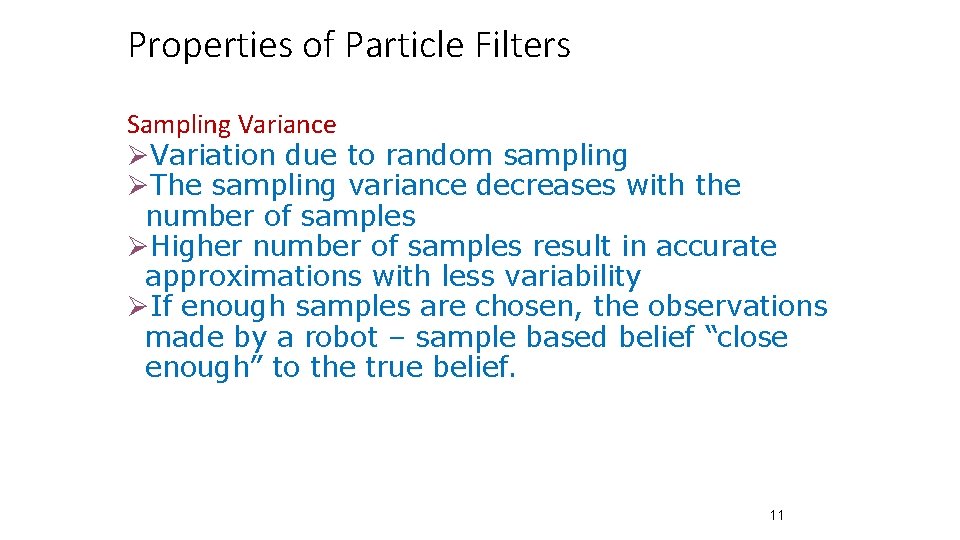
Properties of Particle Filters Sampling Variance ØVariation due to random sampling ØThe sampling variance decreases with the number of samples ØHigher number of samples result in accurate approximations with less variability ØIf enough samples are chosen, the observations made by a robot – sample based belief “close enough” to the true belief. 11

Mobile Robot Particle Filter Video

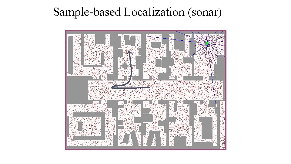
Sample-based Localization (sonar)

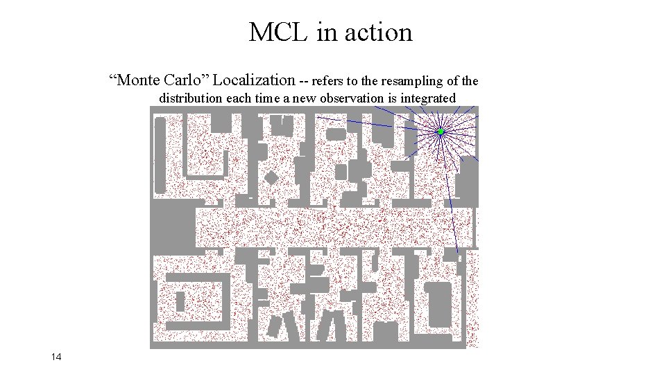
MCL in action “Monte Carlo” Localization -- refers to the resampling of the distribution each time a new observation is integrated 14

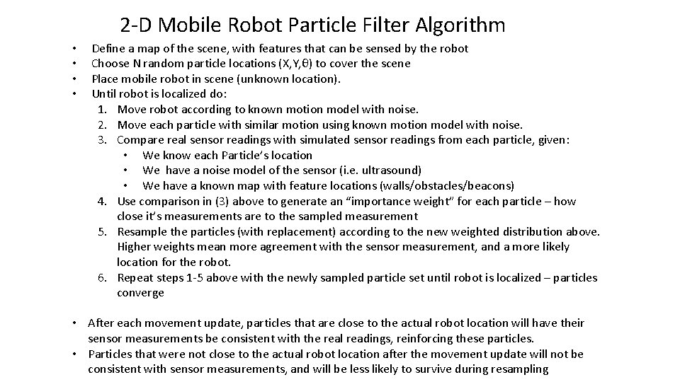
2 -D Mobile Robot Particle Filter Algorithm • • Define a map of the scene, with features that can be sensed by the robot Choose N random particle locations (X, Y, θ) to cover the scene Place mobile robot in scene (unknown location). Until robot is localized do: 1. Move robot according to known motion model with noise. 2. Move each particle with similar motion using known motion model with noise. 3. Compare real sensor readings with simulated sensor readings from each particle, given: • We know each Particle’s location • We have a noise model of the sensor (i. e. ultrasound) • We have a known map with feature locations (walls/obstacles/beacons) 4. Use comparison in (3) above to generate an “importance weight” for each particle – how close it’s measurements are to the sampled measurement 5. Resample the particles (with replacement) according to the new weighted distribution above. Higher weights mean more agreement with the sensor measurement, and a more likely location for the robot. 6. Repeat steps 1 -5 above with the newly sampled particle set until robot is localized – particles converge • After each movement update, particles that are close to the actual robot location will have their sensor measurements be consistent with the real readings, reinforcing these particles. • Particles that were not close to the actual robot location after the movement update will not be consistent with sensor measurements, and will be less likely to survive during resampling

Particle Filter in Python p=[] for i in range(N): p. append(p[i]. location(X, Y, ϴ)) p 2=[] #p is initial particle array with random location of particle (X, Y, ϴ) myrobot=myrobot. move(d. X, d. Y, dϴ) for i in range(N): p 2. append(p[i]. move(d. X, d. Y, dϴ)) #update particle position with movement (rotation, translation) p = p 2 w = [] for i in range(N): #w is importance weight for each particle: P(Z |p[i]) w. append(p[i]. measurement_prob(Z)) #importance weight is how close sensor measurement #at particle location is to actual sensor values p 3 = [] # now resample according to new importance weights …. insert resampling code here to get a new set of particles weighted by their importance p = p 3 # now do this again (starting with myrobot. move() )with the new particle set……

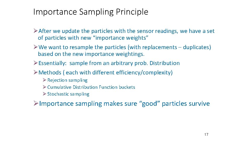
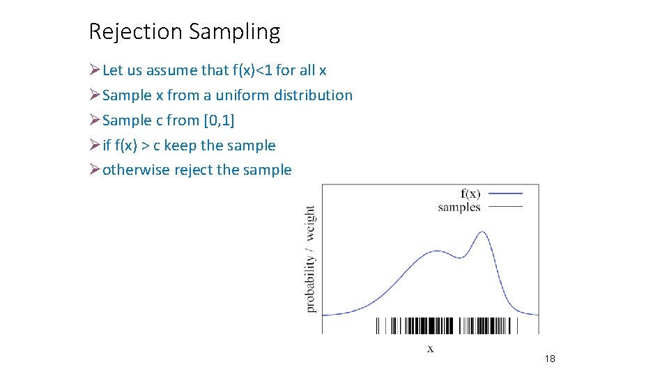
Importance Sampling Principle ØAfter we update the particles with the sensor readings, we have a set of particles with new “importance weights” ØWe want to resample the particles (with replacements – duplicates) based on the new importance weightings. ØEssentially: sample from an arbitrary prob. Distribution ØMethods ( each with different efficiency/complexity) Ø Rejection sampling Ø Cumulative Distribution Function buckets Ø Stochastic sampling ØImportance sampling makes sure “good” particles survive 17

Rejection Sampling ØLet us assume that f(x)<1 for all x ØSample x from a uniform distribution ØSample c from [0, 1] Øif f(x) > c keep the sample Øotherwise reject the sample 18

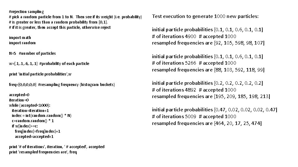
#rejection sampling # pick a random particle from 1 to N. Then see if its weight (i. e. probability) # is greater or less than a random probability from [0, 1]. # if it is greater, then accept this particle, otherwise reject import math import random N=5 #number of particles w=[. 1, . 6, . 1] #probability of each particle print 'initial particle probabilities', w freq=[0, 0, 0] #resampling frequency (histogram buckets) accepted=0 iteration=0 while (accepted<1000): iteration=iteration+1 index = int(random() * N) c=random() * 1 if w[index]>=c: freq[index]=freq[index]+1 accepted=accepted+1 print '# of iterations', iteration, ' # accepted', accepted print 'resampled frequencies are', freq Test execution to generate 1000 new particles: initial particle probabilities [0. 1, 0. 6, 0. 1] # of iterations 4900 # accepted 1000 resampled frequencies are [92, 105, 598, 107] initial particle probabilities [0. 1, 0. 6, 0. 1] # of iterations 5266 # accepted 1000 resampled frequencies are [88, 103, 592, 118, 99] initial particle probabilities [0. 2, 0. 2] # of iterations 4892 # accepted 1000 resampled frequencies are [195, 209, 185, 198, 213] initial particle probabilities [0. 47, 0. 02, 0. 47] # of iterations 5009 # accepted 1000 resampled frequencies are [464, 20, 17, 25, 474]

Simple Particle Filter in Python

Advantages of Particle Filters: Øcan deal with non-linearities, continuous spaces Øcan deal with non-Gaussian noise Øeasy to implement ØPFs focus adaptively on probable regions of state-space ØParallel implementation possible ØCan deal with kidnapped robot problem 21

Drawbacks ØIn order to explore a significant part of the state space, the number of particles should be very large which induces complexity problems not adapted to a real-time implementation. 22

Summary • • • Particle filters are an implementation of recursive Bayesian filtering They represent the posterior by a set of weighted samples. In the context of localization, the particles are propagated according to the motion model. They are then weighted according to the likelihood of the observations. In a re-sampling step, new particles are drawn with a probability proportional to the likelihood of the observation. 23

References 1. Dieter Fox, Wolfram Burgard, Frank Dellaert, Sebastian Thrun, “Monte Carlo Localization: Efficient Position Estimation for Mobile Robots”, Proc. 16 th National Conference on Artificial Intelligence, AAAI’ 99, July 1999 2. Dieter Fox, Wolfram Burgard, Sebastian Thrun, “Markov Localization for Mobile Robots in Dynamic Environments”, J. of Artificial Intelligence Research 11 (1999) 391 -427 3. Sebastian Thrun, “Probabilistic Algorithms in Robotics”, Technical Report CMU-CS-00 -126, School of Computer Science, Carnegie Mellon University, Pittsburgh, USA, 2000 24