Particle Dynamic Systems Visually Illustrating Numeric Integration techniques

Particle Dynamic Systems Visually Illustrating Numeric Integration techniques

Math fun & games n 3 D simulation Physics in games n The problem: providing realistic modeling in real-time n Jeff Lander’s particle simulator in Game Developer magazine illustrates the need for fast, stable numeric integration in games.

Particle System Dynamics n Particles have – Mass – Position – Velocity – May be effected by forces n But do not have spatial extent n Particles experience forces, in our simulator they’re bound by springs

Particle System Dynamics n Each particle is described position, velocity, and force vectors n These vectors form a system of ODEs

Particle System Dynamics n Rewrite each ODE as 2 first order ODEs

Particle System Dynamics n Given the state of the system at some time, t, how can we predict its new state after some step, h, i. e. at time t+h?

A simple solution n Given the state of the system at some time, t, how can we predict its new state after some step, h, i. e. at time t+h? n Euler’s method, a first order Taylor method.

Euler example Consider the IVP: Exact solution: Approximation:

Euler’s Method Graphically

Problems with Euler

Bigger Problems with Euler

BOOM!

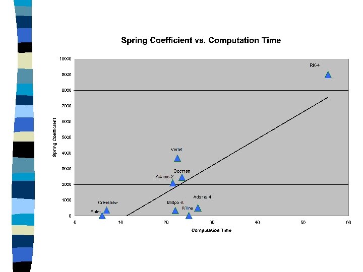
Integrator Criteria n Stable n Computationally fast n low data-storage overhead n Reasonable accuracy (realism)

Alternatives to Euler n Midpoint method n Runge-Kutta 4 n Verlet n Velocity Verlet n Beeman n Adams-Bashforth-Moulton n & more (Gear, symplectics, etc. . )

Velocity Verlet: One Alternative n Begin with two Taylor series expansions: provided that exists and is bounded in the first expansion and exists and is bounded in the second.

An alternative integrator Now we do a reverse Taylor expansion about t+h: Solving this for v(t + h),

An alternative integrator So we have: And, remember from our first velocity expansion, We average these expressions to obtain:

An alternative integrator if f has two bounded derivatives with regard to x, the chain and product rules imply: Then applying the Mean Value Theorem: for some c in (t, t + h). This implies since is bounded.

Velocity Verlet algorithm

Using Velocity Verlet n First, calculate new positions x(t + h) n Next, recompute forces, n Finally, calculate the new velocities, v(t + h)

Velocity Verlet n n n Local error truncation error is O(h 3), assuming f has at least two bounded derivatives. Provides both position and velocity information. Self-starting, no previous data points are needed. More stable than Euler Faster than Runge-Kutta 4

Summary n Particle dynamics simulator provides a tool for visualization of numeric integration techniques. n Qualitative characteristics of algorithm may be observed n Useful for applications such as game development & molecular modeling

Resources This presentation, paper, & related info: http: //titan. wwc. edu/rudy/math/ Original Simulator source by Jeff Lander: http: //www. darwin 3 d. com/gdm 1999. htm#gdm 0399 More information on particle dynamics simulation: http: //www-2. cs. cmu. edu/~baraff/sigcourse/ On Adams-Bashforth-Moulton: Shampine, Lawrence F. and Gordon, M. K. Computer Solution of ODEs: The IVP W. H. Freemand Company (1975): San Francisco, CA. On Velocity Verlet: http: //chemweb. stanford. edu/fall 2001/chem 276/c 276_01_lecture 11. pdf Special Thanks For all his time and help my advisor, Dr. Kenneth Wiggins and for making this presentation possible, Dr. Thomas Thompson Math Department at Walla College

Adams-Bashforth-Moulton n Quadrature n We method need a way to estimate the value of the integral

Adams-Bashforth-Moulton n Construct an interpolating polynomial on the x’ using previous data points.

Adams-Bashforth-Moulton n Formula for integrating the interpolating polynomial can then be constructed n This is the Adams-Bashforth predictor

Adams-Bashforth-Moulton n Using the same technique we construct an implicit formula for the integral n This is the Adams-Moulton corrector

Adams-Bashforth-Moulton n First we predict a new data point using the Adams-Bashforth predictor. n Next, we recompute the force equations based on our prediction. n Then we apply the Adams-Moulton corrector to our previous prediction.

Adams-Bashforth-Moulton n Multi-step (not self starting) n ABM-2 Stability comparable to Velocity Verlet & Beeman n 4 th order less stable than 2 nd order? n Large data-storage overhead