Partially Penetrating Wells By Lauren Cameron Introduction Partially

Partially Penetrating Wells By: Lauren Cameron

Introduction Partially penetrating wells: aquifer is so thick that a fully penetrating well is impractical Increase velocity close to well, extra loss of head, and the effect is inversely related to distance from well (unless the aquifer has obvious anisotropy). Strongest well face Anisotropic aquifers The affect is negligible at distances r > 2 D sqrt(Kb/Kv) *standard methods cannot be used at 2 D sqrt(Kb/Kv) unless allowances are made Assumptions Violated: Well is fully penetrating Flow is horizontal r <

Corrections Different types of aquifers require different modifications Confined and Leaky (steady-state)- Huisman method: Observed drawdowns can be corrected for partial penetration Confined (unsteady-state)- Hantush method: Modification of Theis Method or Jacob Method Leaky (unsteady-state)-Weeks method: Based on Walton and Hantush curve-fitting methods for horizontal flow Unconfined (unsteady-state)- Streltsova curve-fitting or Neuman curve-fitting method Fit data to curves

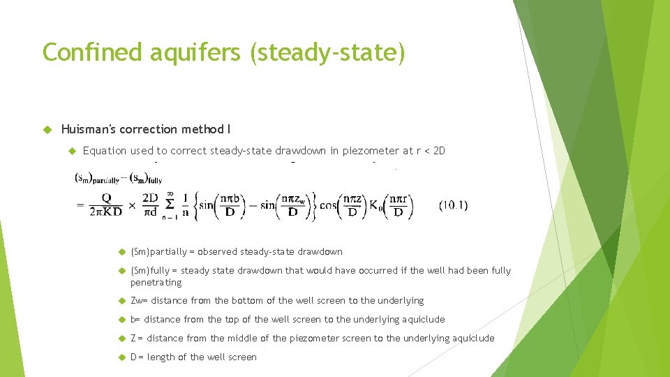
Confined aquifers (steady-state) Huisman's correction method I Equation used to correct steady-state drawdown in piezometer at r < 2 D (Sm)partially = observed steady-state drawdown (Sm)fully = steady state drawdown that would have occurred if the well had been fully penetrating Zw= distance from the bottom of the well screen to the underlying b= distance from the top of the well screen to the underlying aquiclude Z = distance from the middle of the piezometer screen to the underlying aquiclude D = length of the well screen

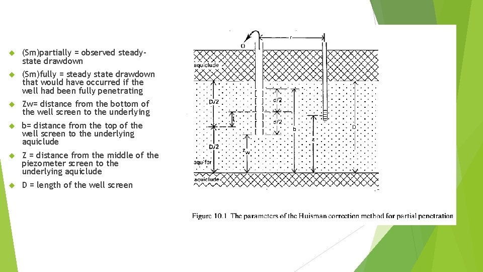
(Sm)partially = observed steadystate drawdown (Sm)fully = steady state drawdown that would have occurred if the well had been fully penetrating Zw= distance from the bottom of the well screen to the underlying b= distance from the top of the well screen to the underlying aquiclude Z = distance from the middle of the piezometer screen to the underlying aquiclude D = length of the well screen

Re: Confined aquifers (steady-state) Assumptions: The assumptions listed at the beginning of Chapter 3, with the exception of the sixth assumption, which is replaced by: The well does not penetrate the entire thickness of the aquifer. The following conditions are added: The flow to the well is in steady state; r > rew = effective radius of the pumped well Remarks Cannot be applied in the immediate vicinity of well where Huisman’s correction method II must be used A few terms of series behind the ∑-sign will generally suffice

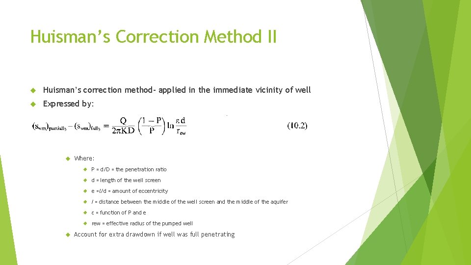
Huisman’s Correction Method II Huisman’s correction method- applied in the immediate vicinity of well Expressed by: Where: P = d/D = the penetration ratio d = length of the well screen e =l/d = amount of eccentricity I = distance between the middle of the well screen and the middle of the aquifer ε = function of P and e rew = effective radius of the pumped well Account for extra drawdown if well was full penetrating

Huisman’s Correction method II Assumptions: The assumptions listed at the beginning of Chapter 3, with the exception of the sixth assumption, which is replaced by: The well does not penetrate the entire thickness of the aquifer. The following conditions are added: The flow to the well is in a steady state; r = rew.

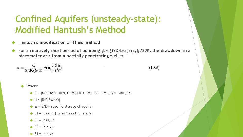
Confined Aquifers (unsteady-state): Modified Hantush’s Method Hantush’s modification of Theis method For a relatively short period of pumping {t < {(2 D-b-a)2(S, )}/20 K, the drawdown in a piezometer at r from a partially penetrating well is Where E(u, (b/r), (d/r), (a/r)) = M(u, B 1) – M(u, B 2) + M(u, B 3) – M(u, B 4) U = (R^2 Ss/4 Kt) Ss = S/D = specific storage of aquifer B 1 = (b+a)/r (for sympols b, d, and a) B 2 = (d+a)/r B 3 = (b-a)/r B 4 = (d-a)/r

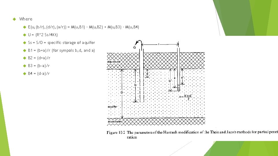
Where E(u, (b/r), (d/r), (a/r)) = M(u, B 1) – M(u, B 2) + M(u, B 3) – M(u, B 4) U = (R^2 Ss/4 Kt) Ss = S/D = specific storage of aquifer B 1 = (b+a)/r (for sympols b, d, and a) B 2 = (d+a)/r B 3 = (b-a)/r B 4 = (d-a)/r

Re: Confined Aquifers (unsteady-state): Modified Hantush’s Method Assumptions: - The assumptions listed at the beginning of Chapter 3, with the exception of the sixth assumption, which is replaced by: The well does not penetrate the entire thickness of the aquifer. The following conditions are added: The flow to the well is in an unsteady state; The time of pumping is relatively short: t < {(2 D-b-a)*(Ss)}/20 K.

Confined Aquifers (unsteady-state): Modified Jacob’s Method Hantush’s modification of the Jacob method can be used if the following assumptions and conditions are satisfied: The assumptions listed at the beginning of Chapter 3, with the exception of the sixth assumption, which is replaced by: The well does not penetrate the entire thickness of the aquifer. The following conditions are added: The flow to the well is in an unsteady state; The time of pumping is relatively long: t > D 2(Ss)/2 K.

Leaky Aquifers (steady-state) The effect of partial penetration is, as a rule, independent of vertical replenishment; therefore, Huisman correction methods I and II can also be applied to leaky aquifers if assumptions are satisfied…

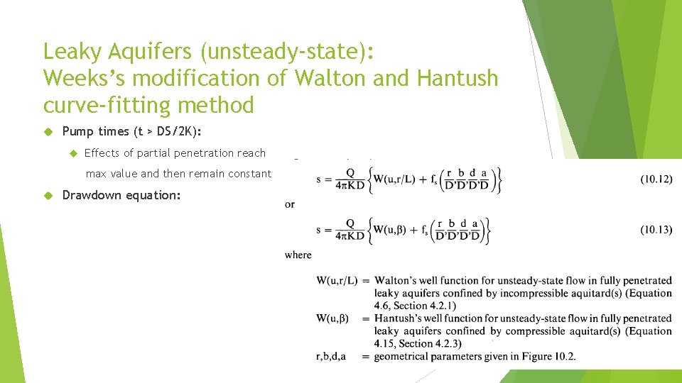
Leaky Aquifers (unsteady-state): Weeks’s modification of Walton and Hantush curve-fitting method Pump times (t > DS/2 K): Effects of partial penetration reach max value and then remain constant Drawdown equation:

Re: Leaky Aquifers (unsteady-state): Weeks’s modification of Walton and Hantush curve-fitting methods The value of f, is constant for a particular well/piezometer configuration and can be determined from Annex 8. 1. With the value of Fs, known, a family of type curves of {W(u, r/L) + fs} or {W(u, p) + f, } versus I/u can be drawn for different values of r/L or p. These can then be matched with the data curve for t > DS/2 K to obtain the hydraulic characteristics of the aquifer.

Re: Leaky Aquifers (unsteady-state): Weeks’s modification of Walton and Hantush curve-fitting methods Assumptions: The Walton curve-fitting method (Section 4. 2. 1) can be used if: The assumptions and conditions in Section 4. 2. 1 are satisfied; A corrected family of type curves (W(u, r/L + fs} is used instead of W(u, r/L); Equation 10. 12 is used instead of Equation 4. 6. The Hantush curve-fitting method (Section 4. 2. 3) can be used if: T > DS/2 K The assumptions and conditions in Section 4. 2. 3 are satisfied; A corrected family of type curves (W(u, p) + fs} is used instead of W(u, p); Equation 10. 13 is used instead of Equation 4. 15.

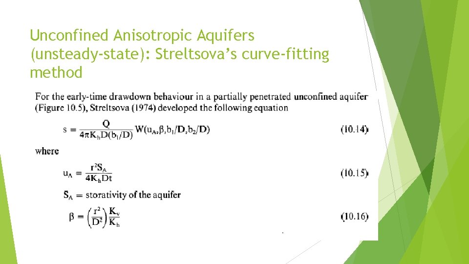
Unconfined Anisotropic Aquifers (unsteady-state): Streltsova’s curve-fitting method

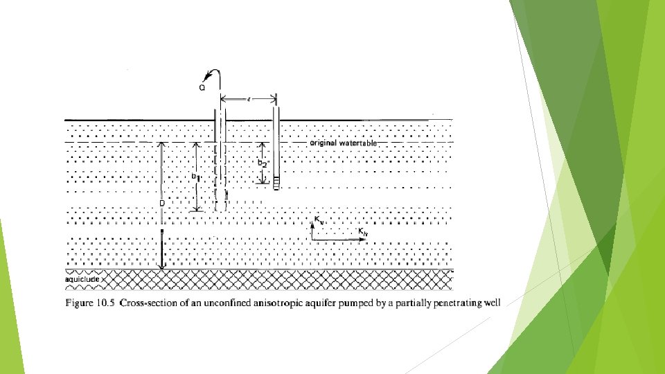
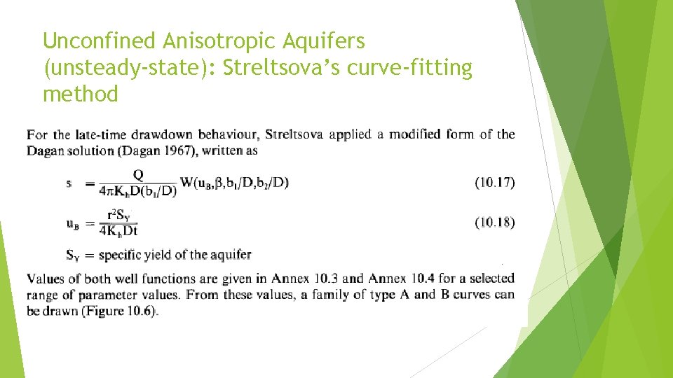
Unconfined Anisotropic Aquifers (unsteady-state): Streltsova’s curve-fitting method

Re: Unconfined Anisotropic Aquifers (unsteady-state): Streltsova’s curve-fitting method Assumptions: The Streltsova curve-fitting method can be used if the following assumptions and conditions are satisfied: The assumptions listed at the beginning of Chapter 3, with the exception of the first, third, sixth and seventh assumptions, which are replaced by The aquifer is homogeneous, anisotropic, and of uniform thickness over the area influenced by the pumping test The well does not penetrate the entire thickness of the aquifer; The aquifer is unconfined and shows delayed water table response. The following conditions are added: The flow to the well is in an unsteady state; SY/SA > 10.

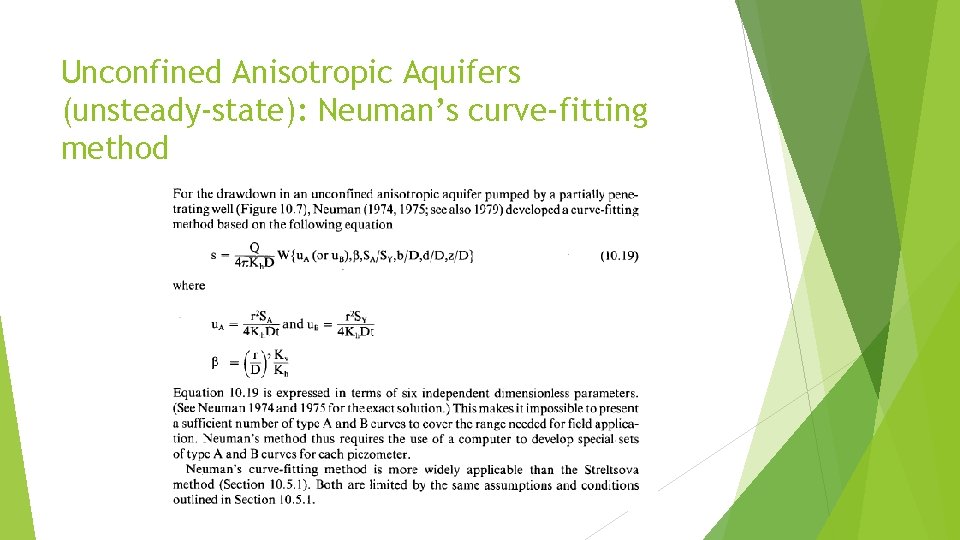
Unconfined Anisotropic Aquifers (unsteady-state): Neuman’s curve-fitting method