Part 6 Synthesis of Heat Exchanger Networks 6

Part 6 Synthesis of Heat Exchanger Networks

6. 1 Sequential Synthesis Minimum Utility Cost

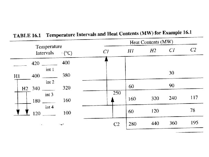
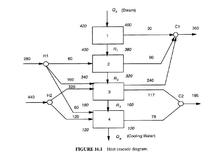
Example 1 H 1 1 400 120 H 2 2 340 120 C 1 1. 5 160 400 C 2 1. 3 100 250

Incidence Matrix of Directed Graph

Material Balance Around a Node

Minimum Cost Flow Problem

Transshipment Problem The transportation problem is a special case of the minimum cost flow problem, corresponding to a network with arcs going only from supply to demand nodes. The more general problem allows for arbitrary network configuration, so that flow from a supply node may progress through several intermediate nodes before reaching its destination. The more general problem is often termed the transshipment problem.

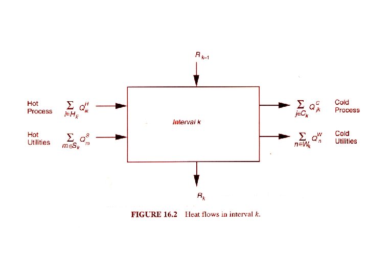
Heat Balances around Temperature Intervals (Warehouses)

Transshipment Model Total utility consumption rate LP problem

60 30 0 123 225

Index Sets

Condensed Transshipment Model Total utility cost Known

Remarks •

Example 2 (The transshipment model can be generalized to consider multiple utilities to minimize total utility cost. ) H 1 FCp (MW/K) 2. 5 Tin (K) 400 Tout (K) 320 H 2 3. 8 370 320 C 1 2. 0 300 420 C 2 2. 0 300 370 HP Steam: 500 K, $80/k. W-yr LP Steam: 380 K, $50/k. W-yr Cooling Water: 300 K, $20/k. W-yr HRAT: 10 K

HP steam 500 K 380 K

Sequential Synthesis Minimum Utility Cost with Constrained Matches (The transshipment model can be expanded so as to handle constraints on matches. )

Example 1 H 1 1 400 120 H 2 2 340 120 C 1 1. 5 160 400 C 2 1. 3 100 250

Expanded heat cascade!

Basic Ideas

Two Possible Heat. Exchange Options 1. Hot stream i and cold stream j are both present in interval k. 2. Cold stream j is present in interval k, but hot stream i is only present at higher temperature interval.

Hot stream i and cold stream j are both present in interval k

Cold stream j is present in interval 3, but hot stream i is only present at interval 2

Index Sets

Expanded Transshipment Model

Match Constraints

Modified Example 1 H 1 1 400 120 H 2 2 340 120 C 1 1. 5 160 400 C 2 1. 3 100 250

60 30 0 123 225

Condensed Transshipment Model The annual utility cost: $9, 300, 000.

Expanded heat cascade!

Expanded Transshipment Model

Expanded Transshipment Model Annual Utility Cost: $15, 300, 000 Heating Utility Load: 120 MW Cooling Utility Load: 285 MW

Sequential Synthesis Prediction of optimal matches for minimizing the unit number in HEN

Objective Function q=1, 2, …. , NP+1

Heat Balances The constraints in the expanded transshipment model can be modified for the present model: 1. The heat contents of the utility streams are given. 2. The common index i can be used for hot process and utility streams; The common index j can be used for cold process and utility streams.

Expanded Transshipment Model

Modification of Expanded Transshipment Model

Heat Balances

Logical Constraints

Solution

Example 1 Fcp (MW/C) Tin (C) Tout (C) H 1 1 400 120 H 2 2 340 120 C 1 1. 5 160 400 C 2 1. 3 100 250 Steam: 500 C Cooling water: 20 – 30 C Minimum recovery approach temperature (HRAT): 20 C

Condensed Transshipment Model

Pinch

MILP (i)

MILP (ii)

Solution

Manual Synthesis

Alternative Solution

Solve MILP without Partition

Only 5 units! One less than the previous two!

Sequential Synthesis Automatic Generation of Network Structures

Basic Ideas of Superstructure • Each exchanger in HEN corresponds to a match predicted by the MILP model (with or without pinch partition). • Each exchanger in HEN should also have as heat duty the one predicted by MILP. • The superstructure will contain the stream interconnections among the aforementioned exchangers that can potentially define all configurations. • The flow rates and temperatures of stream interconnections in superstructure will be treated as unknowns that must be determined.

Example 3 Stream Tin (K) Tout (K) Fcp (k. W/K) Heat Load (k. W) h (k. W/m^2 K) Cost ($/k. Wyr) H 1 440 350 22 1980 2. 0 - C 1 349 430 20 1620 2. 0 - C 2 320 368 7. 5 360 0. 67 - S 1 500 - 0 120 W 1 300 320 - 0 1. 0 20

Step 1 & Step 2

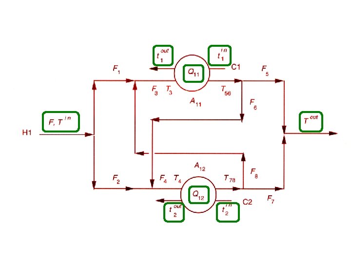
Superstructure for hot stream H 1

Embedded Alternative Configurations • • H 1 -C 1 and H 1 -C 2 in series H 1 -C 2 and H 1 -C 1 in series H 1 -C 1 and H 1 -C 2 in parallel with bypass to H 1 -C 2 • H 1 -C 1 and H 1 -C 2 in parallel with bypass to H 1 -C 1

Parameters and Unknowns

Equality Constraints

Inequality Constraints

Objective Function

Solution