Part 5 Response of Linear Systems 6 Linear

Part 5 Response of Linear Systems 6. Linear Filtering of a Random Signals 7. Power Spectrum Analysis 8. Linear Estimation and Prediction Filters 9. Mean-Square Estimation 1

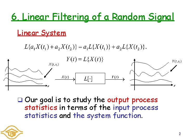
6. Linear Filtering of a Random Signal Linear System q Our goal is to study the output process statistics in terms of the input process statistics and the system function. 2

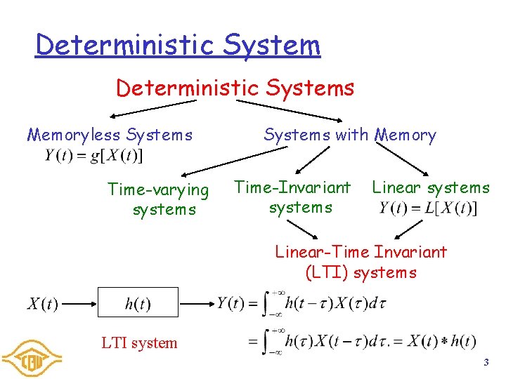
Deterministic Systems Memoryless Systems Time-varying systems Systems with Memory Time-Invariant systems Linear-Time Invariant (LTI) systems LTI system 3

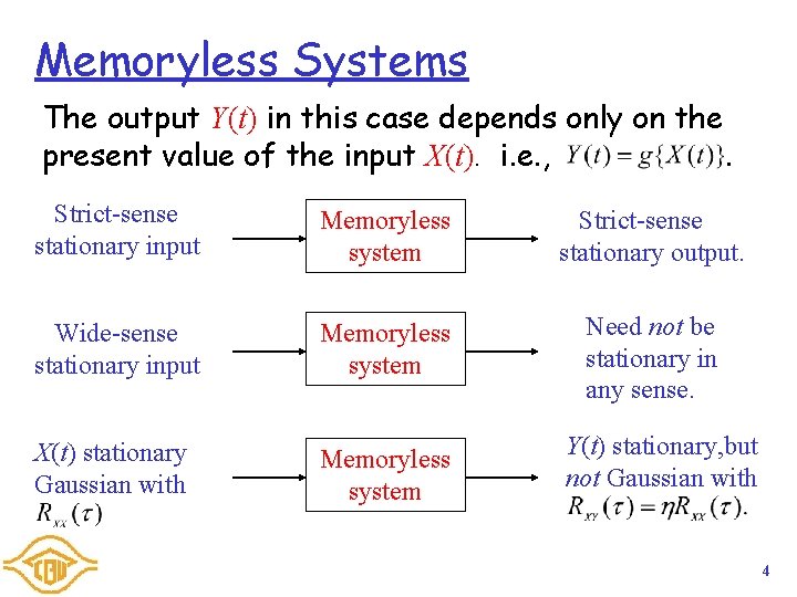
Memoryless Systems The output Y(t) in this case depends only on the present value of the input X(t). i. e. , . Strict-sense stationary input Memoryless system Strict-sense stationary output. Wide-sense stationary input Memoryless system Need not be stationary in any sense. X(t) stationary Gaussian with Memoryless system Y(t) stationary, but not Gaussian with 4

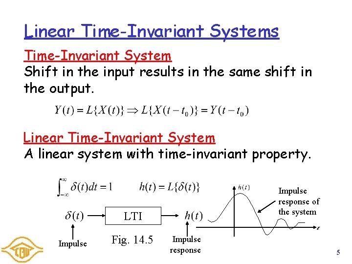
Linear Time-Invariant Systems Time-Invariant System Shift in the input results in the same shift in the output. Linear Time-Invariant System A linear system with time-invariant property. Impulse response of the system LTI Impulse Fig. 14. 5 Impulse response 5

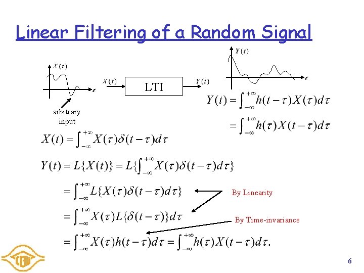
Linear Filtering of a Random Signal LTI arbitrary input By Linearity By Time-invariance 6

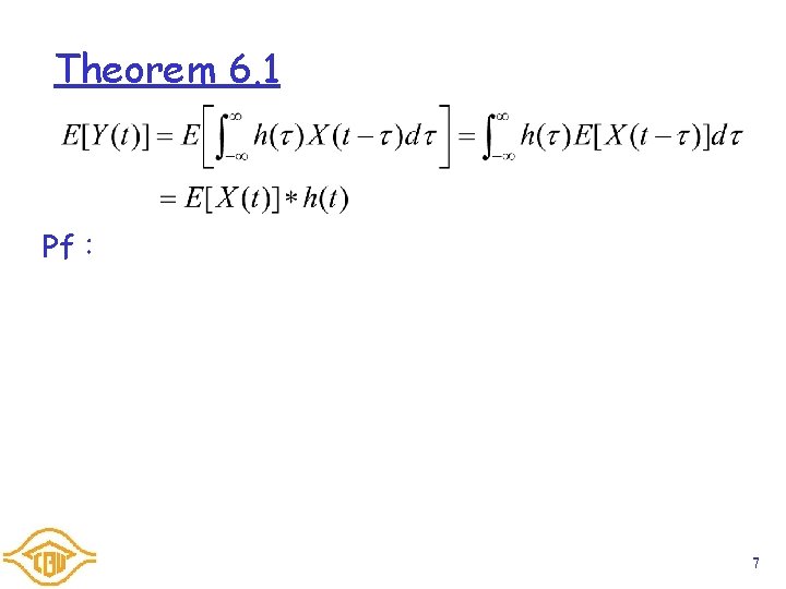
Theorem 6. 1 Pf： 7

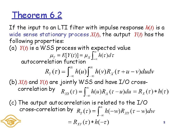
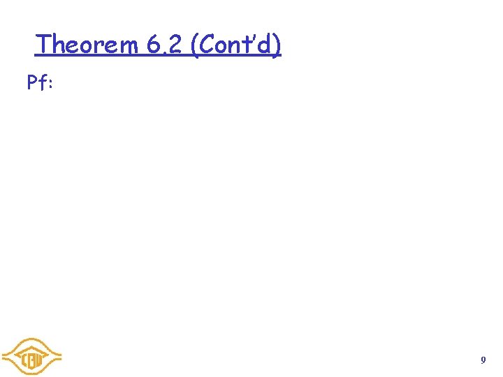
Theorem 6. 2 If the input to an LTI filter with impulse response h(t) is a wide sense stationary process X(t), the output Y(t) has the following properties: (a) Y(t) is a WSS process with expected value autocorrelation function (b) X(t) and Y(t) are jointly WSS and have I/O crosscorrelation by (c) The output autocorrelation is related to the I/O cross-correlation by 8

Theorem 6. 2 (Cont’d) Pf: 9

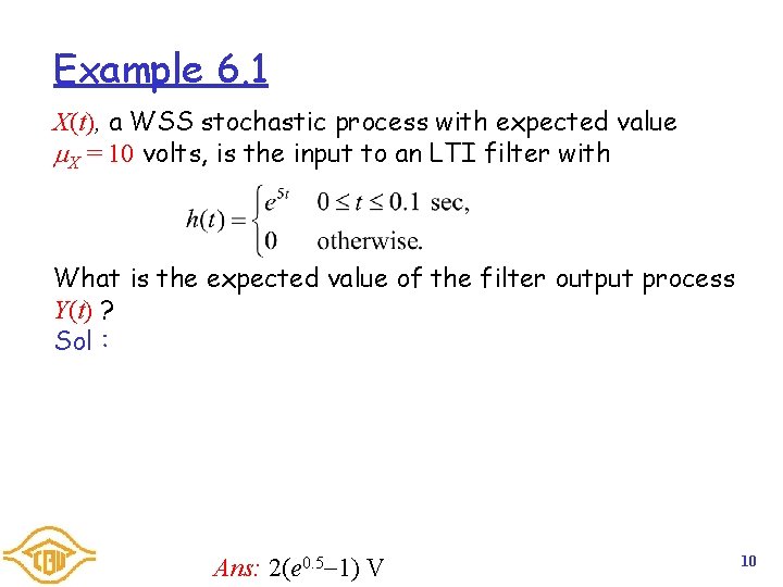
Example 6. 1 X(t), a WSS stochastic process with expected value X = 10 volts, is the input to an LTI filter with What is the expected value of the filter output process Y(t) ? Sol： Ans: 2(e 0. 5 1) V 10

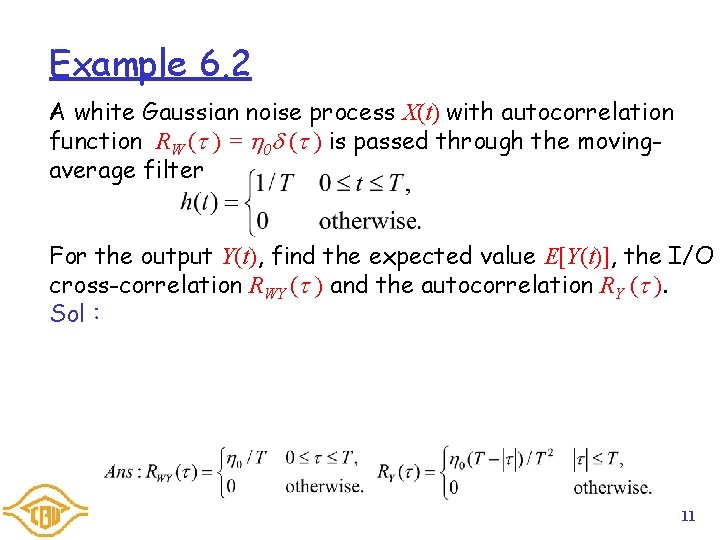
Example 6. 2 A white Gaussian noise process X(t) with autocorrelation function RW ( ) = 0 ( ) is passed through the movingaverage filter For the output Y(t), find the expected value E[Y(t)], the I/O cross-correlation RWY ( ) and the autocorrelation RY ( ). Sol： 11

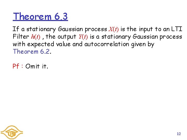
Theorem 6. 3 If a stationary Gaussian process X(t) is the input to an LTI Filter h(t) , the output Y(t) is a stationary Gaussian process with expected value and autocorrelation given by Theorem 6. 2. Pf：Omit it. 12

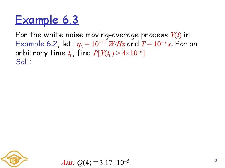
Example 6. 3 For the white noise moving-average process Y(t) in Example 6. 2, let 0 = 10 15 W/Hz and T = 10 3 s. For an arbitrary time t 0, find P[Y(t 0) > 4 10 6]. Sol： Ans: Q(4) = 3. 17 10 5 13

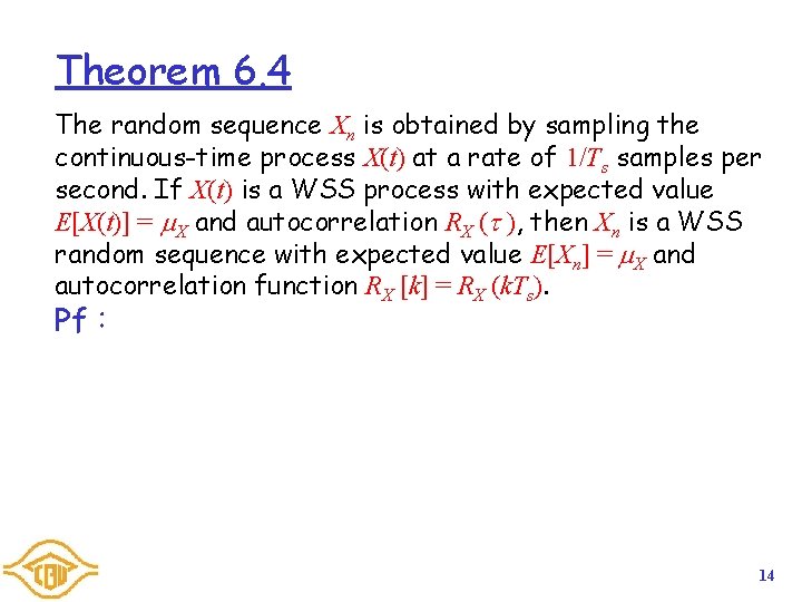
Theorem 6. 4 The random sequence Xn is obtained by sampling the continuous-time process X(t) at a rate of 1/Ts samples per second. If X(t) is a WSS process with expected value E[X(t)] = X and autocorrelation RX ( ), then Xn is a WSS random sequence with expected value E[Xn] = X and autocorrelation function RX [k] = RX (k. Ts). Pf： 14

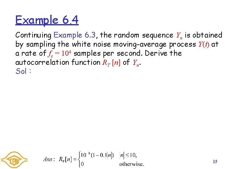
Example 6. 4 Continuing Example 6. 3, the random sequence Yn is obtained by sampling the white noise moving-average process Y(t) at a rate of fs = 104 samples per second. Derive the autocorrelation function RY [n] of Yn. Sol： 15

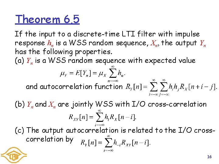
Theorem 6. 5 If the input to a discrete-time LTI filter with impulse response hn is a WSS random sequence, Xn, the output Yn has the following properties. (a) Yn is a WSS random sequence with expected value and autocorrelation function (b) Yn and Xn are jointly WSS with I/O cross-correlation (c) The output autocorrelation is related to the I/O crosscorrelation by 16

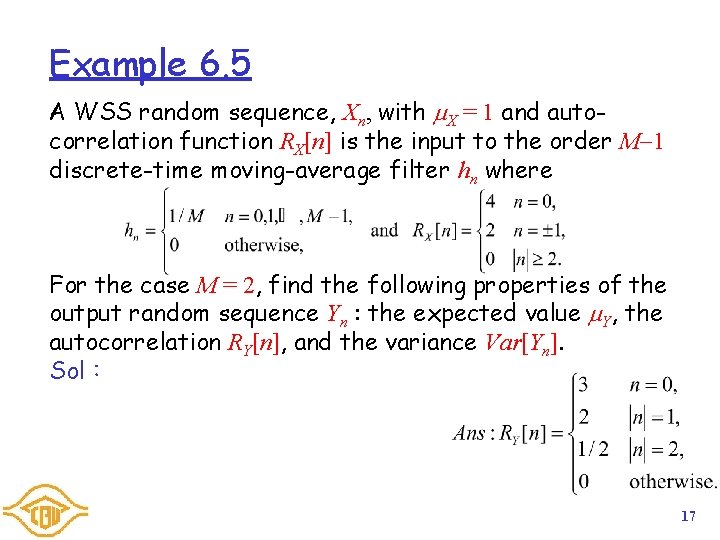
Example 6. 5 A WSS random sequence, Xn, with X = 1 and autocorrelation function RX[n] is the input to the order M 1 discrete-time moving-average filter hn where For the case M = 2, find the following properties of the output random sequence Yn : the expected value Y, the autocorrelation RY[n], and the variance Var[Yn]. Sol： 17

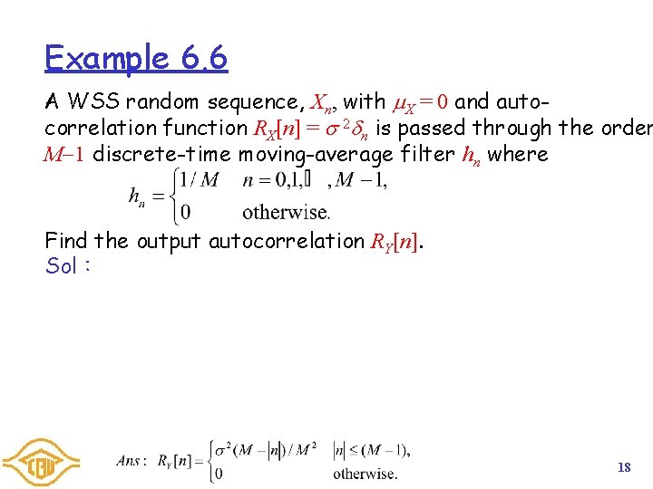
Example 6. 6 A WSS random sequence, Xn, with X = 0 and autocorrelation function RX[n] = 2 n is passed through the order M 1 discrete-time moving-average filter hn where Find the output autocorrelation RY[n]. Sol： 18

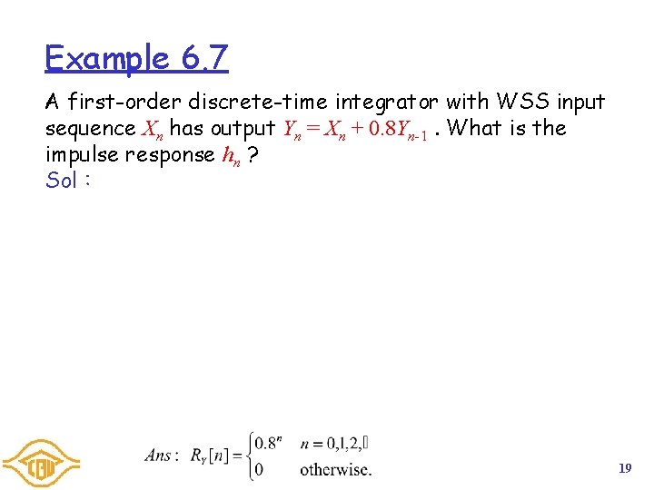
Example 6. 7 A first-order discrete-time integrator with WSS input sequence Xn has output Yn = Xn + 0. 8 Yn-1. What is the impulse response hn ? Sol： 19

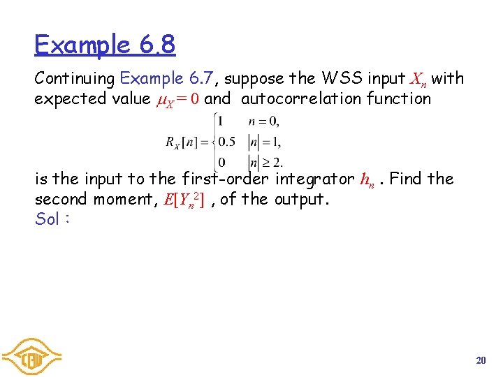
Example 6. 8 Continuing Example 6. 7, suppose the WSS input Xn with expected value X = 0 and autocorrelation function is the input to the first-order integrator hn. Find the second moment, E[Yn 2] , of the output. Sol： 20

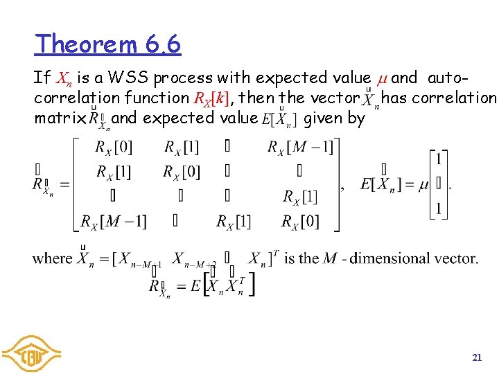
Theorem 6. 6 If Xn is a WSS process with expected value and autocorrelation function RX[k], then the vector has correlation matrix and expected value given by 21

Example 6. 9 The WSS sequence Xn has autocorrelation function RX[n] as given in Example 6. 5. Find the correlation matrix of Sol： 22

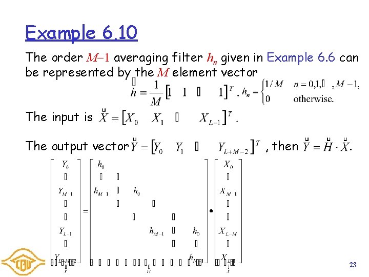
Example 6. 10 The order M 1 averaging filter hn given in Example 6. 6 can be represented by the M element vector The input is The output vector , then . 23

6. Linear Filtering of a Random Signals 7. Power Spectrum Analysis 8. Linear Estimation and Prediction Filters 9. Mean-Square Estimation 24

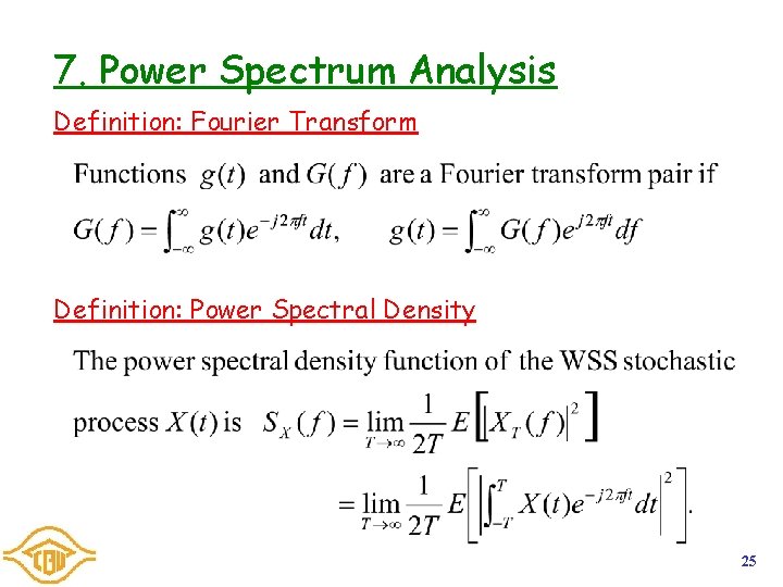
7. Power Spectrum Analysis Definition: Fourier Transform Definition: Power Spectral Density 25

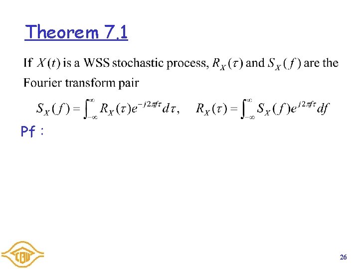
Theorem 7. 1 Pf： 26

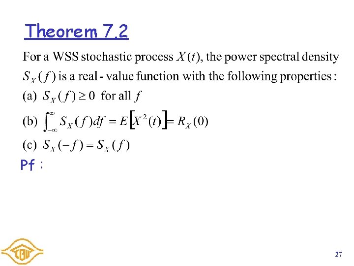
Theorem 7. 2 Pf： 27

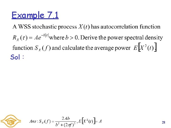
Example 7. 1 Sol： 28

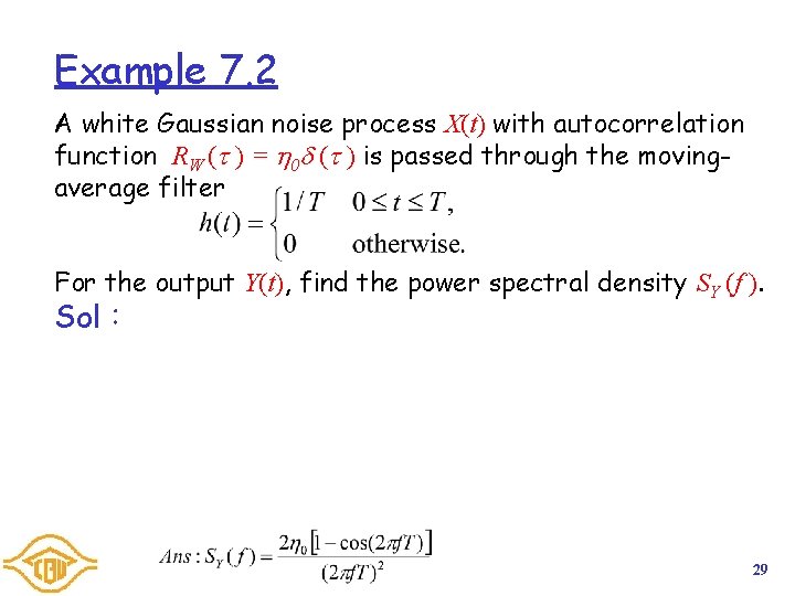
Example 7. 2 A white Gaussian noise process X(t) with autocorrelation function RW ( ) = 0 ( ) is passed through the movingaverage filter For the output Y(t), find the power spectral density SY (f ). Sol： 29

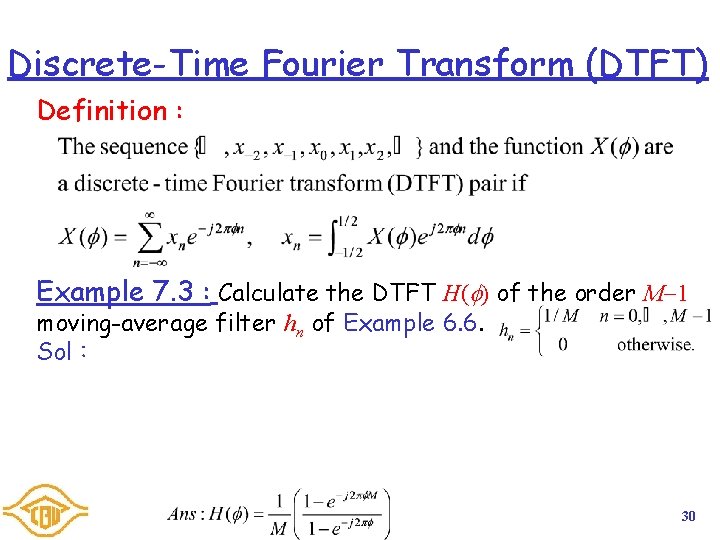
Discrete-Time Fourier Transform (DTFT) Definition : Example 7. 3 : Calculate the DTFT H( ) of the order M 1 moving-average filter hn of Example 6. 6. Sol： 30

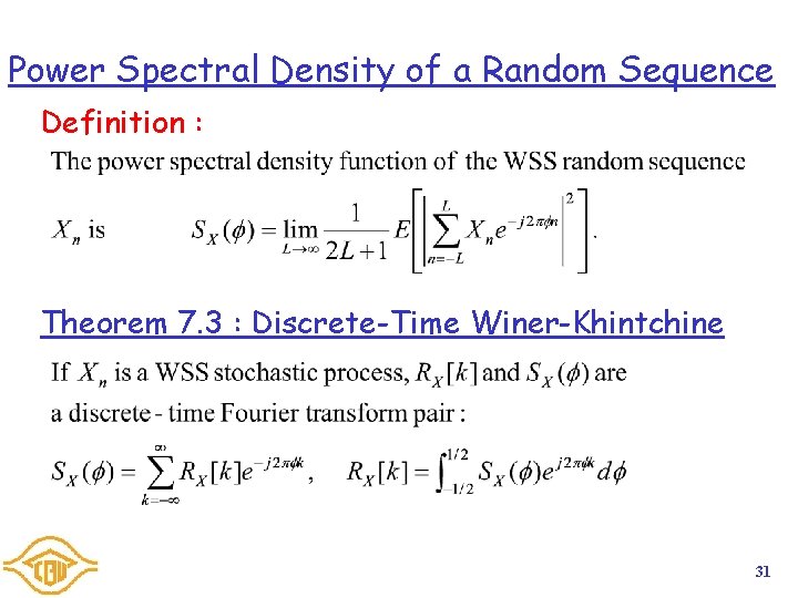
Power Spectral Density of a Random Sequence Definition : Theorem 7. 3 : Discrete-Time Winer-Khintchine 31

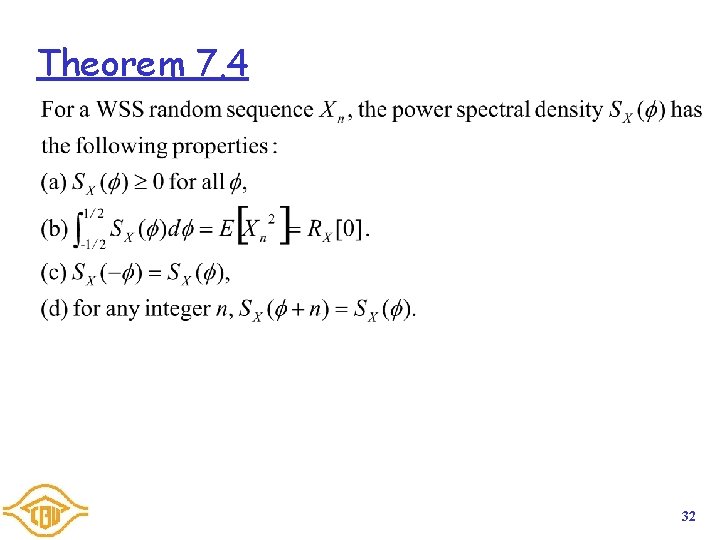
Theorem 7. 4 32

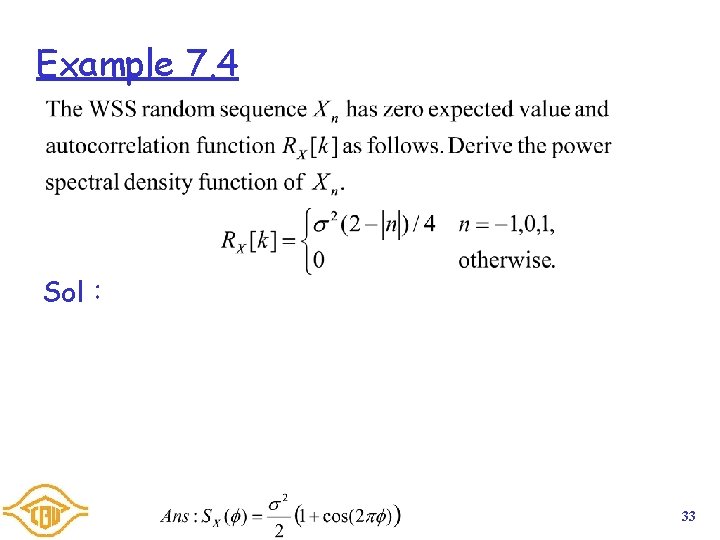
Example 7. 4 Sol： 33

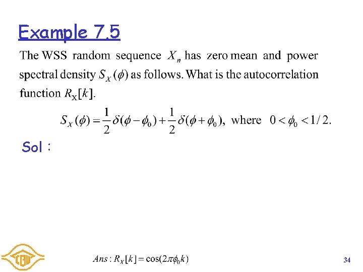
Example 7. 5 Sol： 34

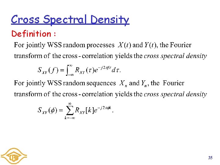
Cross Spectral Density Definition : 35

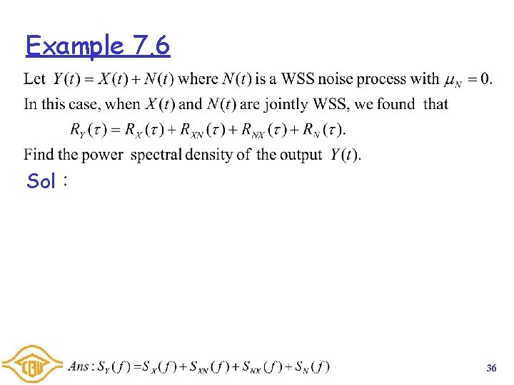
Example 7. 6 Sol： 36

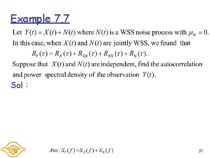
Example 7. 7 Sol： 37

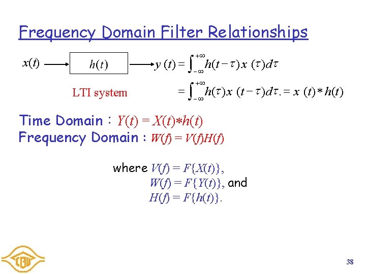
Frequency Domain Filter Relationships +¥ y (t ) = ò ¥ h(t ) x ( )d x(t) LTI system +¥ = ò h( ) x (t )d . = x (t ) h(t ) ¥ Time Domain：Y(t) = X(t) h(t) Frequency Domain : W(f) = V(f)H(f) where V(f) = F{X(t)}, W(f) = F{Y(t)}, and H(f) = F{h(t)}. 38

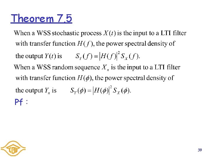
Theorem 7. 5 Pf： 39

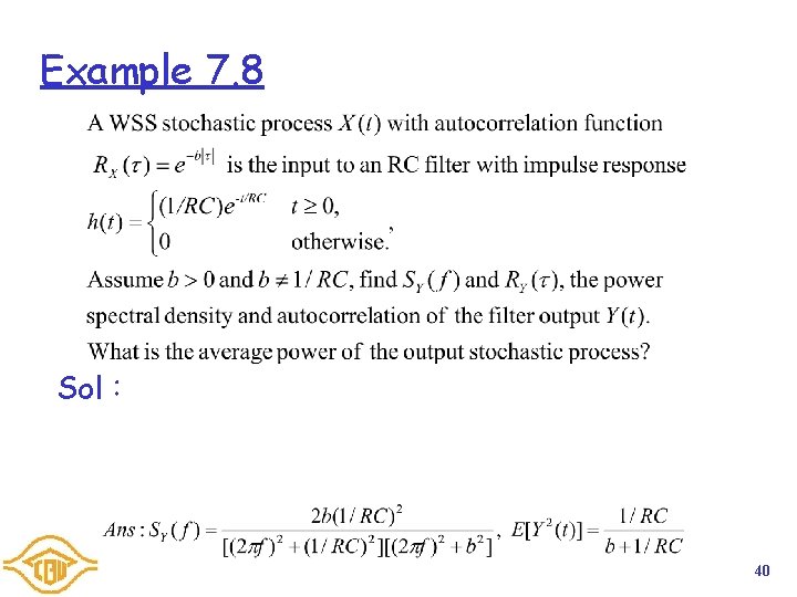
Example 7. 8 Sol： 40

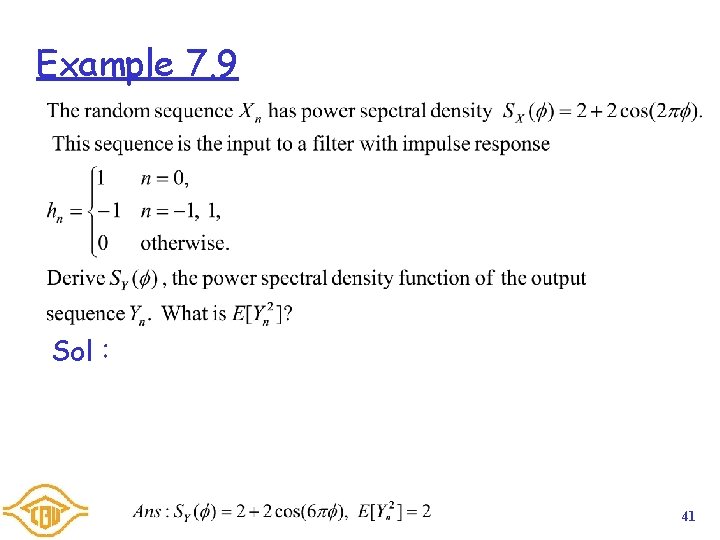
Example 7. 9 Sol： 41

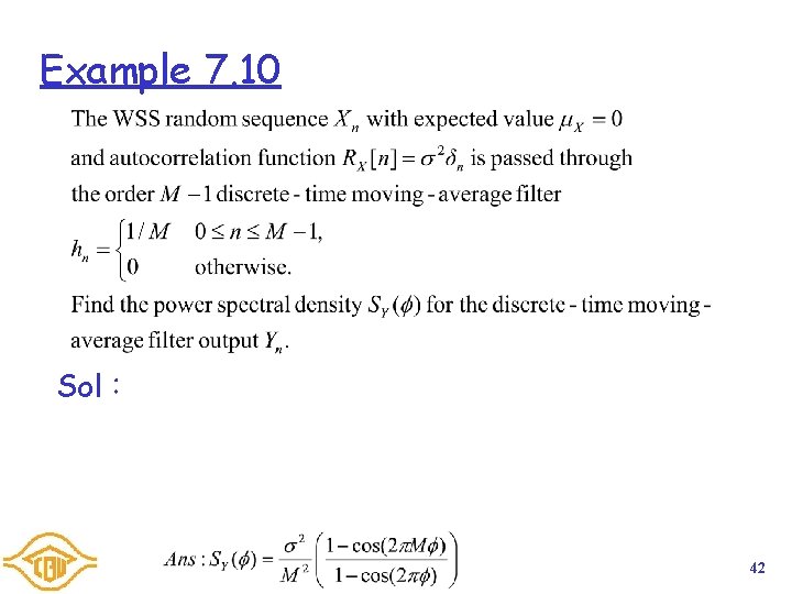
Example 7. 10 Sol： 42

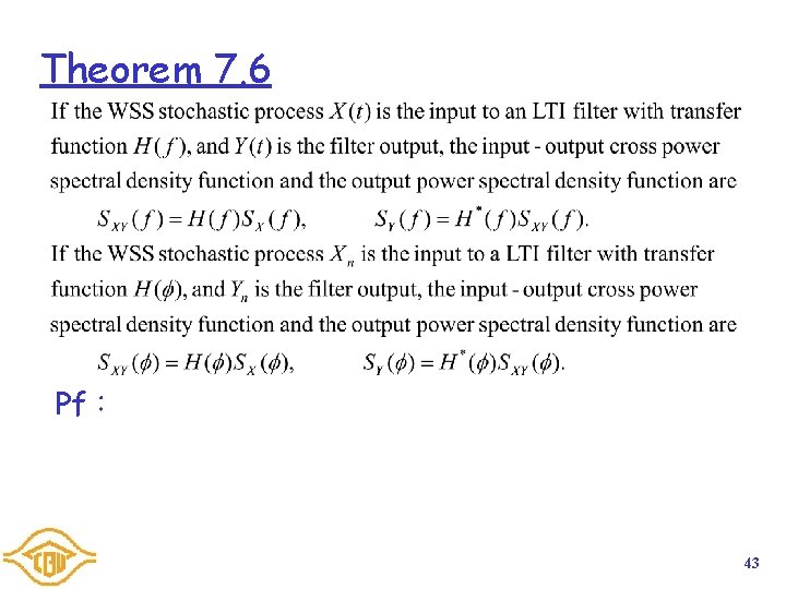
Theorem 7. 6 Pf： 43

I/O Correlation and Spectral Density Functions R X ( ) RX[k] h(t) hn RXY( ) RXY[k] h(-t) h-n R Y ( ) RY[k] Time Domain SX(f) SX( ) H(f) H( ) SXY(f) SXY( ) H*(f) SY(f) H*( ) SY( ) Frequency Domain 44

6. Linear Filtering of a Random Signals 7. Power Spectrum Analysis 8. Linear Estimation and Prediction Filters 9. Mean-Square Estimation 45

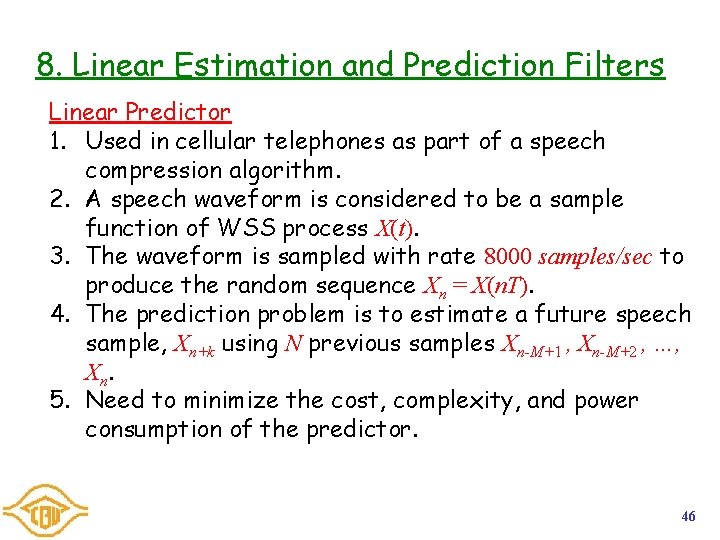
8. Linear Estimation and Prediction Filters Linear Predictor 1. Used in cellular telephones as part of a speech compression algorithm. 2. A speech waveform is considered to be a sample function of WSS process X(t). 3. The waveform is sampled with rate 8000 samples/sec to produce the random sequence Xn = X(n. T). 4. The prediction problem is to estimate a future speech sample, Xn+k using N previous samples Xn-M+1 , Xn-M+2 , …, Xn. 5. Need to minimize the cost, complexity, and power consumption of the predictor. 46

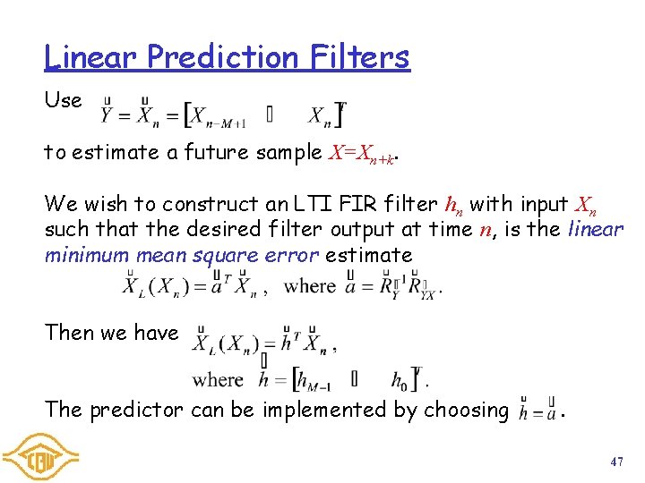
Linear Prediction Filters Use to estimate a future sample X=Xn+k. We wish to construct an LTI FIR filter hn with input Xn such that the desired filter output at time n, is the linear minimum mean square error estimate Then we have The predictor can be implemented by choosing . 47

Theorem 8. 1 Let Xn be a WSS random process with expected value E[Xn] = 0 and autocorrelation function RX[k]. The minimum mean square error linear filter of order M 1, for predicting Xn+k at time n is the filter such that where is called as the cross-correlation matrix. 48

Example 8. 1 Xn be a WSS random sequence with E[Xn] = 0 and autocorrelation function RX[k]= ( 0. 9)|k|. For M = 2 samples, find , the coefficients of the optimum linear predictor for X = Xn+1, given. What is the optimum linear predictor of Xn+1 , given Xn 1 and Xn. What is the mean square error of the optimal predictor? Sol： 49

Theorem 8. 2 If the random sequence Xn has a autocorrelation function RX[n]= b|k| RX[0], the optimum linear predictor of Xn+k, given the M previous samples is and the minimum mean square error is Pf： . 50

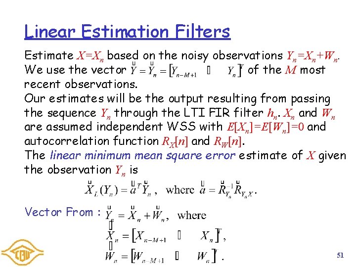
Linear Estimation Filters Estimate X=Xn based on the noisy observations Yn=Xn+Wn. We use the vector of the M most recent observations. Our estimates will be the output resulting from passing the sequence Yn through the LTI FIR filter hn. Xn and Wn are assumed independent WSS with E[Xn]=E[Wn]=0 and autocorrelation function RX[n] and RW[n]. The linear minimum mean square error estimate of X given the observation Yn is Vector From : 51

Theorem 8. 3 Let Xn and Wn be independent WSS random processes with E[Xn]=E[Wn]=0 and autocorrelation function RX[k] and RW[k]. Let Yn=Xn+Wn. The minimum mean square error linear estimation filter of Xn of order M 1 given the input Yn is given by such that 52

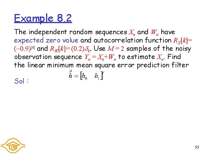
Example 8. 2 The independent random sequences Xn and Wn have expected zero value and autocorrelation function RX[k]= ( 0. 9)|k| and RW[k]= (0. 2) k. Use M = 2 samples of the noisy observation sequence Yn = Xn+Wn to estimate Xn. Find the linear minimum mean square error prediction filter Sol： 53

6. Linear Filtering of a Random Signals 7. Power Spectrum Analysis 8. Linear Estimation and Prediction Filters 9. Mean-Square Estimation 54

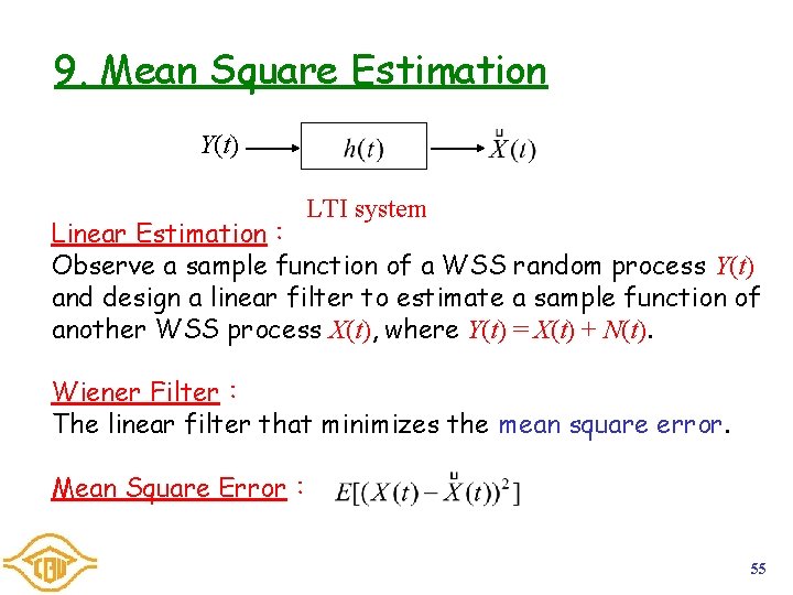
9. Mean Square Estimation Y(t) LTI system Linear Estimation： Observe a sample function of a WSS random process Y(t) and design a linear filter to estimate a sample function of another WSS process X(t), where Y(t) = X(t) + N(t). Wiener Filter： The linear filter that minimizes the mean square error. Mean Square Error： 55

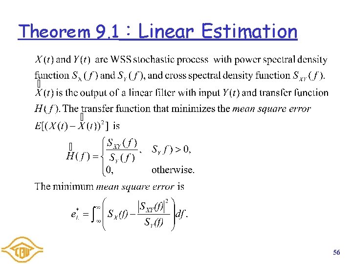
Theorem 9. 1：Linear Estimation 56

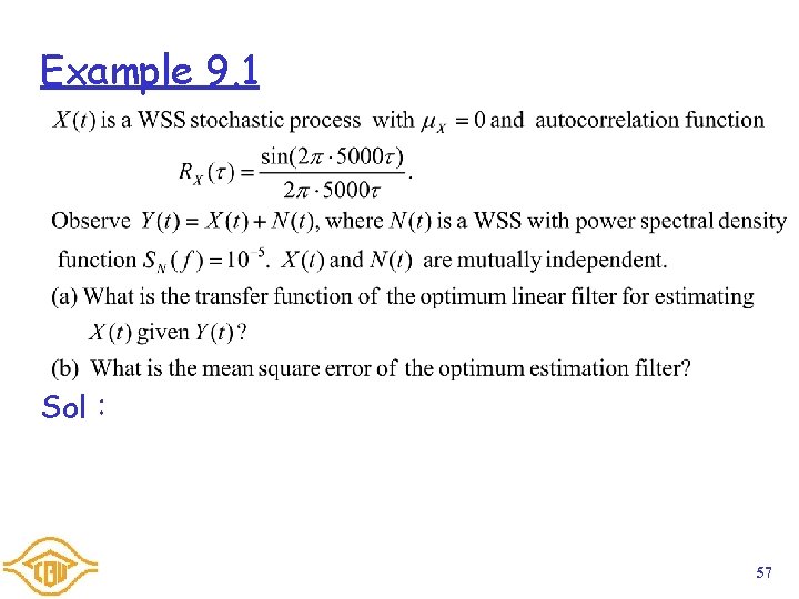
Example 9. 1 Sol： 57