Part 4 ADVANCED SVMbased LEARNING METHODS Vladimir Cherkassky

Part 4: ADVANCED SVM-based LEARNING METHODS Vladimir Cherkassky University of Minnesota cherk 001@umn. edu Presented at Tech Tune Ups, ECE Dept, June 1, 2011 Electrical and Computer Engineering 1

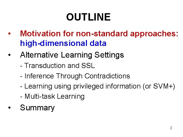
OUTLINE • • Motivation for non-standard approaches: high-dimensional data Alternative Learning Settings - Transduction and SSL - Inference Through Contradictions - Learning using privileged information (or SVM+) - Multi-task Learning • Summary 2

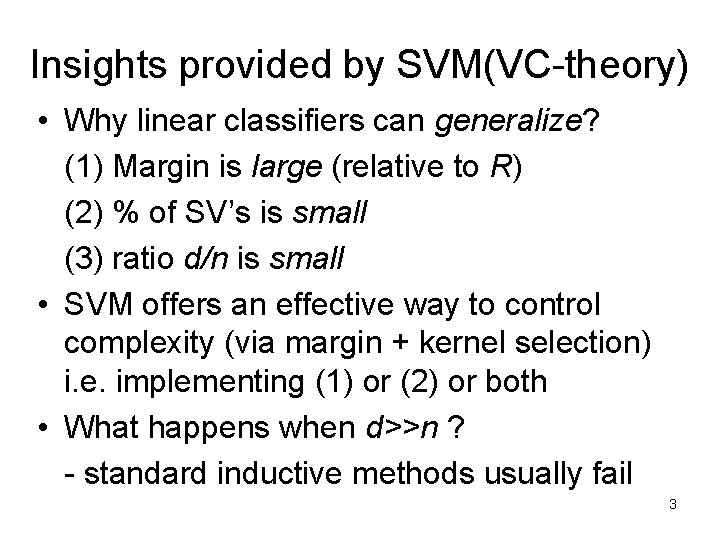
Insights provided by SVM(VC-theory) • Why linear classifiers can generalize? (1) Margin is large (relative to R) (2) % of SV’s is small (3) ratio d/n is small • SVM offers an effective way to control complexity (via margin + kernel selection) i. e. implementing (1) or (2) or both • What happens when d>>n ? - standard inductive methods usually fail 3

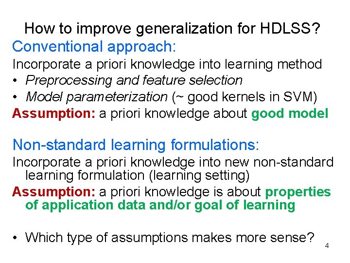
How to improve generalization for HDLSS? Conventional approach: Incorporate a priori knowledge into learning method • Preprocessing and feature selection • Model parameterization (~ good kernels in SVM) Assumption: a priori knowledge about good model Non-standard learning formulations: Incorporate a priori knowledge into new non-standard learning formulation (learning setting) Assumption: a priori knowledge is about properties of application data and/or goal of learning • Which type of assumptions makes more sense? 4

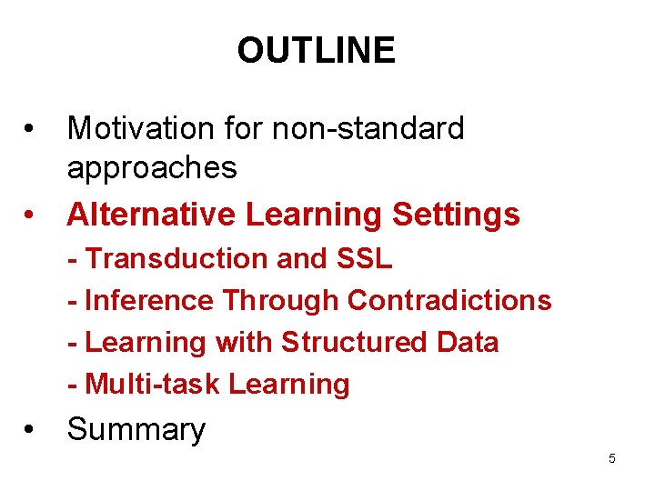
OUTLINE • Motivation for non-standard approaches • Alternative Learning Settings - Transduction and SSL - Inference Through Contradictions - Learning with Structured Data - Multi-task Learning • Summary 5

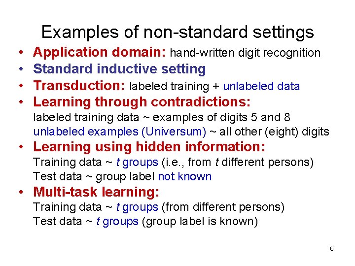
Examples of non-standard settings • • Application domain: hand-written digit recognition Standard inductive setting Transduction: labeled training + unlabeled data Learning through contradictions: labeled training data ~ examples of digits 5 and 8 unlabeled examples (Universum) ~ all other (eight) digits • Learning using hidden information: Training data ~ t groups (i. e. , from t different persons) Test data ~ group label not known • Multi-task learning: Training data ~ t groups (from different persons) Test data ~ t groups (group label is known) 6

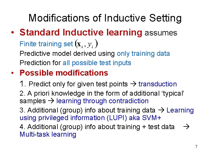
Modifications of Inductive Setting • Standard Inductive learning assumes Finite training set Predictive model derived using only training data Prediction for all possible test inputs • Possible modifications 1. Predict only for given test points transduction 2. A priori knowledge in the form of additional ‘typical’ samples learning through contradiction 3. Additional (group) info about training data Learning using privileged information (LUPI) aka SVM+ 4. Additional (group) info about training + test data Multi-task learning 7

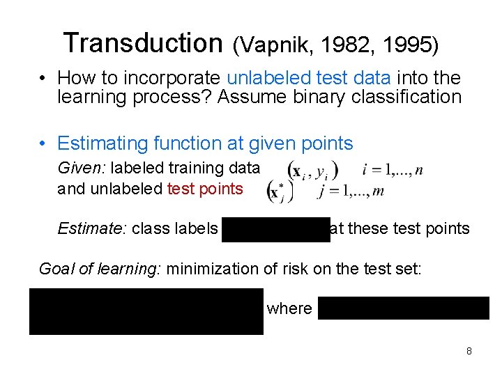
Transduction (Vapnik, 1982, 1995) • How to incorporate unlabeled test data into the learning process? Assume binary classification • Estimating function at given points Given: labeled training data and unlabeled test points Estimate: class labels at these test points Goal of learning: minimization of risk on the test set: where 8

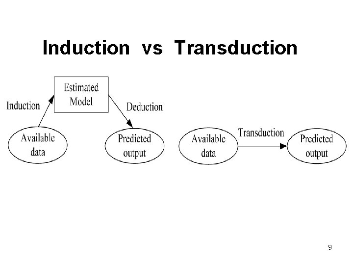
Induction vs Transduction 9

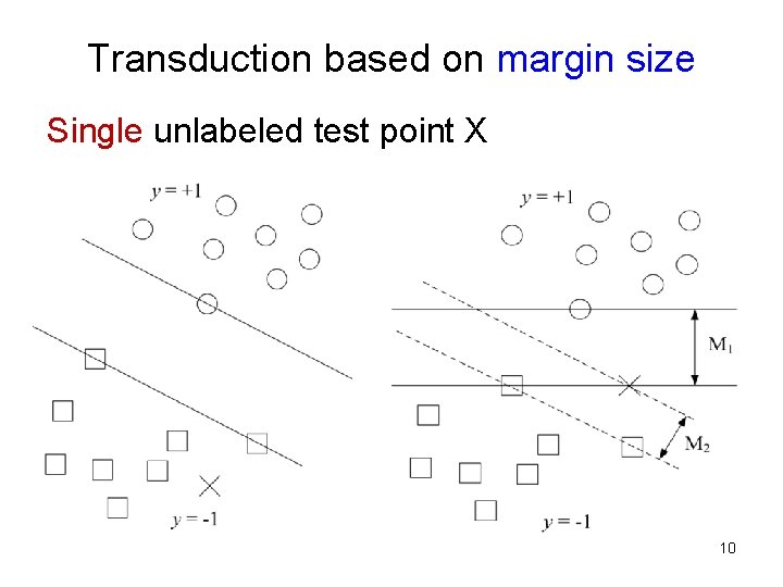
Transduction based on margin size Single unlabeled test point X 10

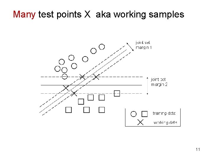
Many test points X aka working samples 11

Transduction based on margin size • Binary classification, linear parameterization, joint set of (training + working) samples • Two objectives of transductive learning: (TL 1) separate labeled training data using a largemargin hyperplane (as in standard inductive SVM) (TL 2) separating (explain) working data set using a large-margin hyperplane. 12

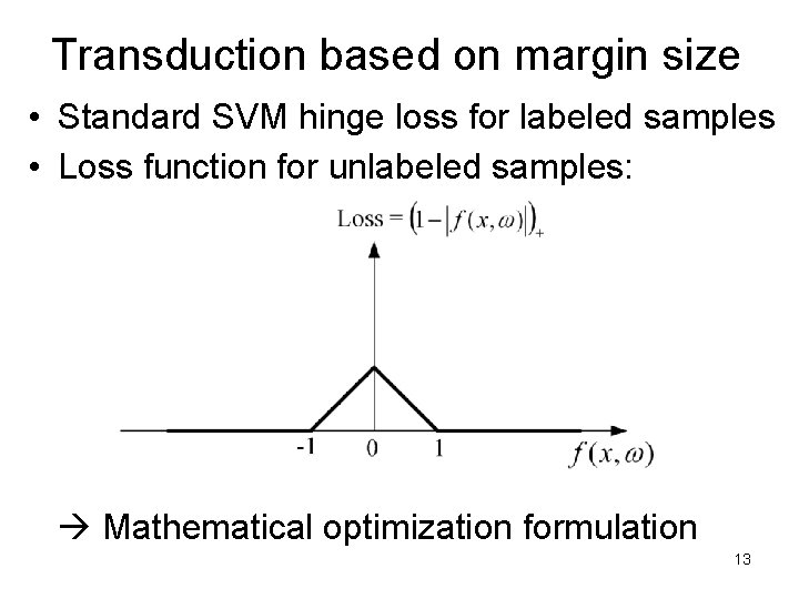
Transduction based on margin size • Standard SVM hinge loss for labeled samples • Loss function for unlabeled samples: Mathematical optimization formulation 13

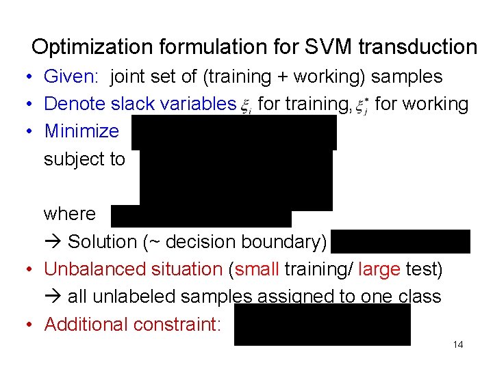
Optimization formulation for SVM transduction • Given: joint set of (training + working) samples • Denote slack variables for training, for working • Minimize subject to where Solution (~ decision boundary) • Unbalanced situation (small training/ large test) all unlabeled samples assigned to one class • Additional constraint: 14

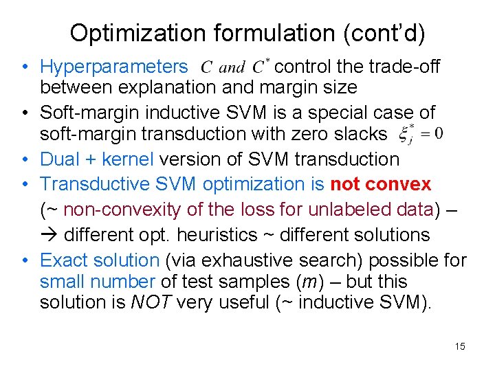
Optimization formulation (cont’d) • Hyperparameters control the trade-off between explanation and margin size • Soft-margin inductive SVM is a special case of soft-margin transduction with zero slacks • Dual + kernel version of SVM transduction • Transductive SVM optimization is not convex (~ non-convexity of the loss for unlabeled data) – different opt. heuristics ~ different solutions • Exact solution (via exhaustive search) possible for small number of test samples (m) – but this solution is NOT very useful (~ inductive SVM). 15

Many applications for transduction • Text categorization: classify word documents into a number of predetermined categories • Email classification: Spam vs non-spam • Web page classification • Image database classification • All these applications: - high-dimensional data - small labeled training set (human-labeled) - large unlabeled test set 16

Example application • Prediction of molecular bioactivity for drug discovery • Training data~1, 909; test~634 samples • Input space ~ 139, 351 -dimensional • Prediction accuracy: SVM induction ~74. 5%; transduction ~ 82. 3% Ref: J. Weston et al, KDD cup 2001 data analysis: prediction of molecular bioactivity for drug design – binding to thrombin, Bioinformatics 2003 17

Semi-Supervised Learning (SSL) • Labeled data + unlabeled data Model • Similar to transduction (but not the same): - Goal 1 ~ prediction for unlabeled samples - Goal 2 ~ estimate an inductive model • Many algorithms • Applications similar to transduction • Typically - Transduction works better for HDLSS - SSL works better for low-dimensional data 18

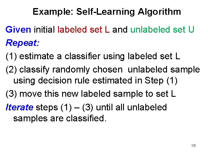
Example: Self-Learning Algorithm Given initial labeled set L and unlabeled set U Repeat: (1) estimate a classifier using labeled set L (2) classify randomly chosen unlabeled sample using decision rule estimated in Step (1) (3) move this new labeled sample to set L Iterate steps (1) – (3) until all unlabeled samples are classified. 19

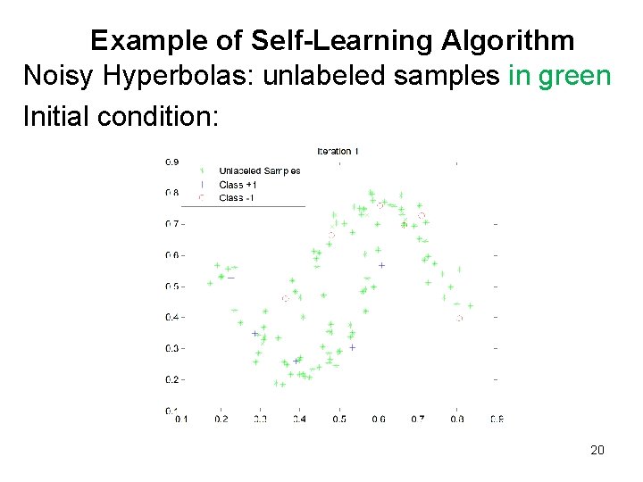
Example of Self-Learning Algorithm Noisy Hyperbolas: unlabeled samples in green Initial condition: 20

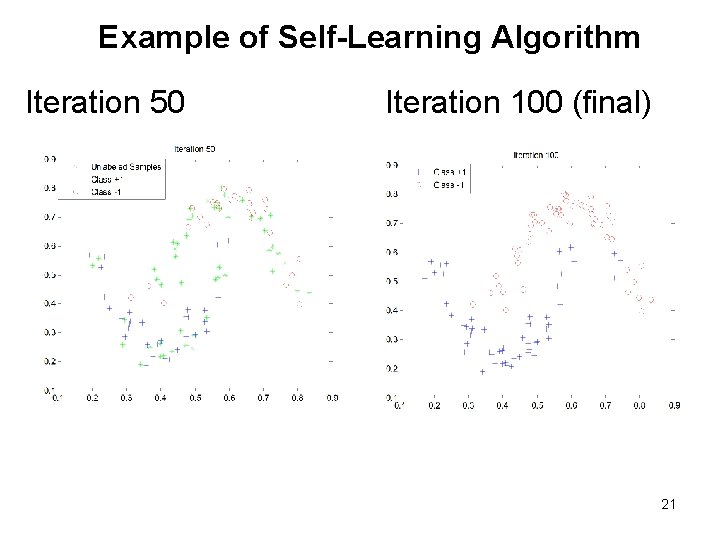
Example of Self-Learning Algorithm Iteration 50 Iteration 100 (final) 21

Inference through contradiction (Vapnik 2006) • Motivation: what is a priori knowledge? - info about the space of admissible models - info about admissible data samples • Labeled training samples + unlabeled samples from the Universum • Universum samples encode info about the region of input space (where application data lives): - Usually from a different distribution than training/test data • Examples of the Universum data • Large improvement for small training samples 22

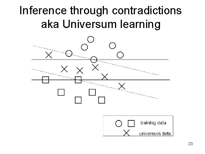
Inference through contradictions aka Universum learning 23

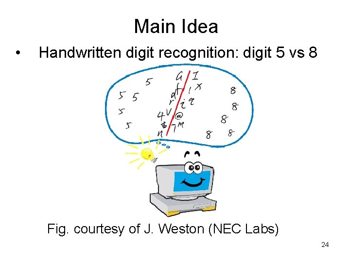
Main Idea • Handwritten digit recognition: digit 5 vs 8 Fig. courtesy of J. Weston (NEC Labs) 24

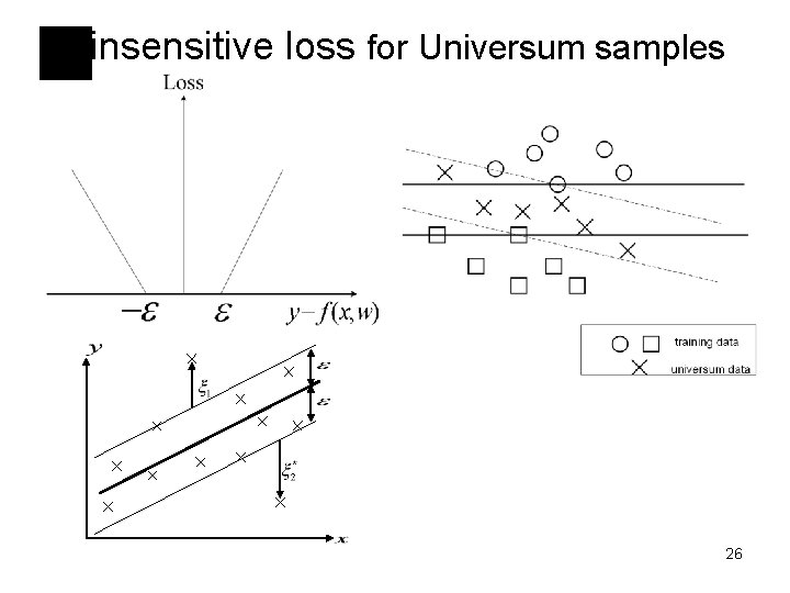
Learning with the Universum • Inductive setting for binary classification Given: labeled training data and unlabeled Universum samples Goal of learning: minimization of prediction risk (as in standard inductive setting) • Balance between two goals: - explain labeled training data using large-margin hyperplane - achieve maximum falsifiability ~ max # contradictions on the Universum Math optimization formulation (extension of SVM) 25

-insensitive loss for Universum samples 26

Random averaging Universum Class 1 Average Class -1 Hyper-plane 27

Random Averaging for digits 5 and 8 • Two randomly selected examples • Universum sample: 28

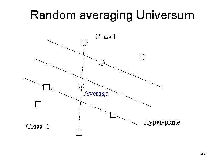
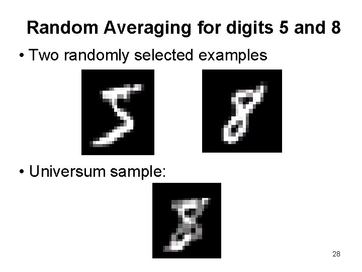
Application Study (Vapnik, 2006) • Binary classification of handwritten digits 5 and 8 • For this binary classification problem, the following Universum sets had been used: U 1: randomly selected digits (0, 1, 2, 3, 4, 6, 7, 9) U 2: randomly mixing pixels from images 5 and 8 U 3: average of randomly selected examples of 5 and 8 Training set size tried: 250, 500, … 3, 000 samples Universum set size: 5, 000 samples • Prediction error: improved over standard SVM, i. e. for 500 training samples: 1. 4% vs 2% (SVM) 29

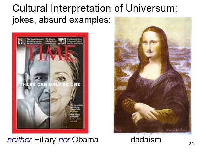
Cultural Interpretation of Universum: jokes, absurd examples: neither Hillary nor Obama dadaism 30

Application Study: predicting gender of human faces • Binary classification setting • Difficult problem: dimensionality ~ large (10 K - 20 K) labeled sample size ~ small (~ 10 - 20) • Humans perform very well for this task • Issues: - possible improvement (vs standard SVM) - how to choose ‘good’ Universum? - model parameter tuning 31

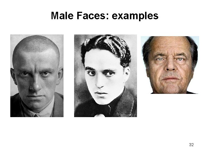
Male Faces: examples 32

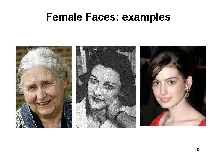
Female Faces: examples 33

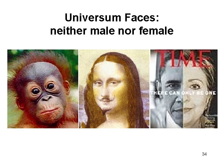
Universum Faces: neither male nor female 34

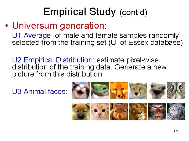
Empirical Study (cont’d) • Universum generation: U 1 Average: of male and female samples randomly selected from the training set (U. of Essex database) U 2 Empirical Distribution: estimate pixel-wise distribution of the training data. Generate a new picture from this distribution U 3 Animal faces: 35

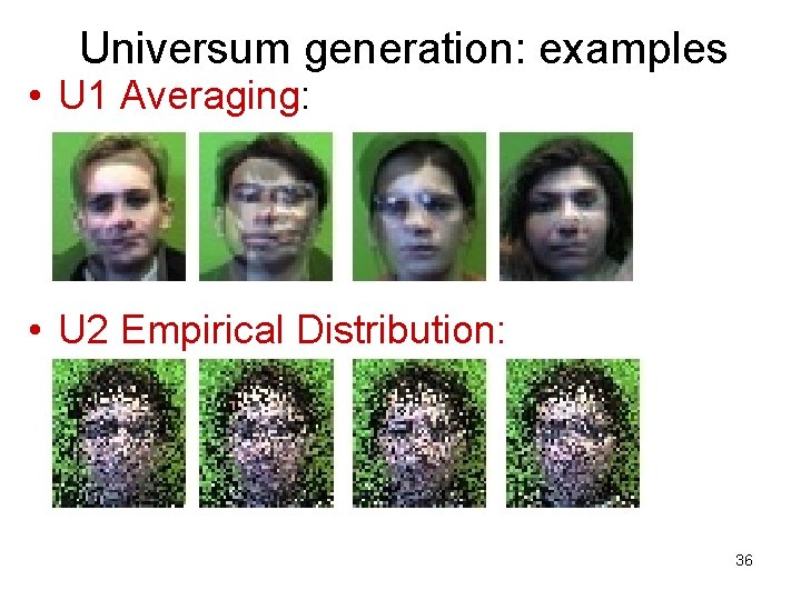
Universum generation: examples • U 1 Averaging: • U 2 Empirical Distribution: 36

Results of gender classification • Classification accuracy: improves vs standard SVM by ~ 2% with U 1 Universum, and by ~ 1% with U 2 Universum. • Universum by averaging gives better results for this problem, when number of Universum samples N = 500 or 1, 000 37

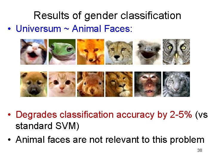
Results of gender classification • Universum ~ Animal Faces: • Degrades classification accuracy by 2 -5% (vs standard SVM) • Animal faces are not relevant to this problem 38

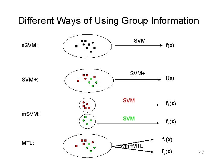
Learning with Structured Data(Vapnik, 2006) • Application: Handwritten digit recognition Labeled training data provided by t persons (t >1) Goal 1: find a classifier that will generalize well for future samples generated by these persons ~ Learning with Structured Data or Learning using Hidden Information Goal 2: find t classifiers with generalization (for each person) ~ Multi-Task Learning (MTL) • Application: Medical diagnosis Labeled training data provided by t groups of patients (t >1), say men and women (t = 2) Goal 1: estimate a classifier to predict/diagnose a disease using training data from t groups of patients ~ LWSD Goal 2: find t classifiers specialized for each group of patients ~ MTL 39

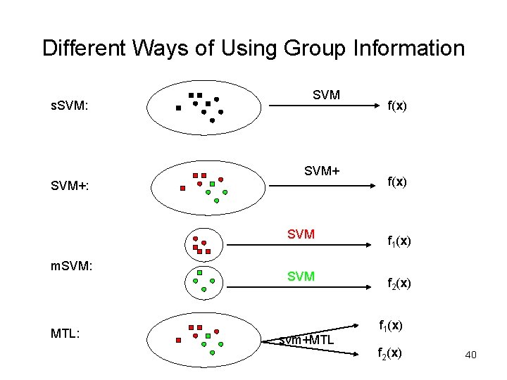
Different Ways of Using Group Information s. SVM: SVM+: m. SVM: MTL: f(x) SVM f 1(x) SVM f 2(x) svm+MTL f 1(x) f 2(x) 40

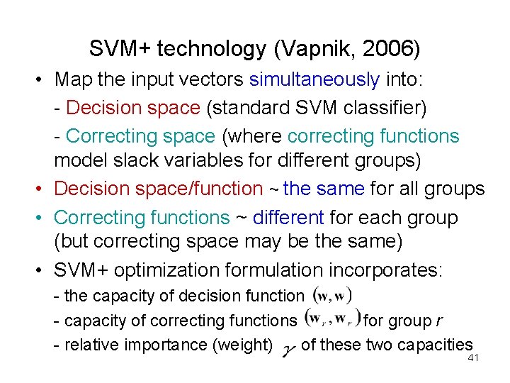
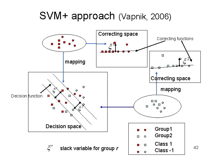
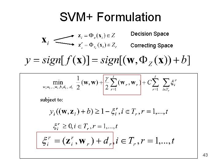
SVM+ technology (Vapnik, 2006) • Map the input vectors simultaneously into: - Decision space (standard SVM classifier) - Correcting space (where correcting functions model slack variables for different groups) • Decision space/function ~ the same for all groups • Correcting functions ~ different for each group (but correcting space may be the same) • SVM+ optimization formulation incorporates: - the capacity of decision function - capacity of correcting functions for group r - relative importance (weight) of these two capacities 41

SVM+ approach (Vapnik, 2006) Correcting space Correcting functions mapping Correcting space mapping Decision function Decision space slack variable for group r Group 1 Group 2 Class 1 Class -1 42

SVM+ Formulation Decision Space Correcting Space subject to: 43

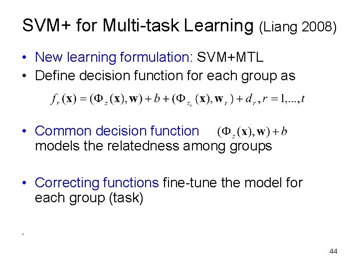
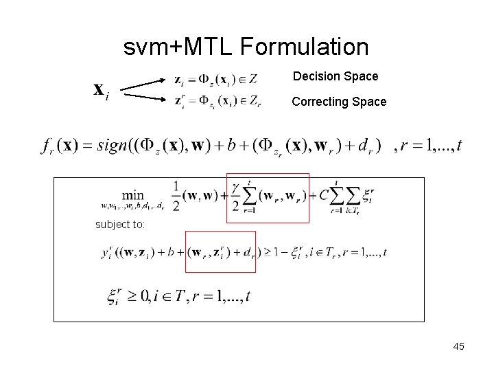
SVM+ for Multi-task Learning (Liang 2008) • New learning formulation: SVM+MTL • Define decision function for each group as • Common decision function models the relatedness among groups • Correcting functions fine-tune the model for each group (task). 44

svm+MTL Formulation Decision Space Correcting Space subject to: 45

Empirical Validation • • Different ways of using group info different learning settings: - which one yields better generalization? - how performance is affected by sample size? Empirical comparisons: - synthetic data set 46

Different Ways of Using Group Information s. SVM: SVM+: m. SVM: MTL: f(x) SVM f 1(x) SVM f 2(x) svm+MTL f 1(x) f 2(x) 47

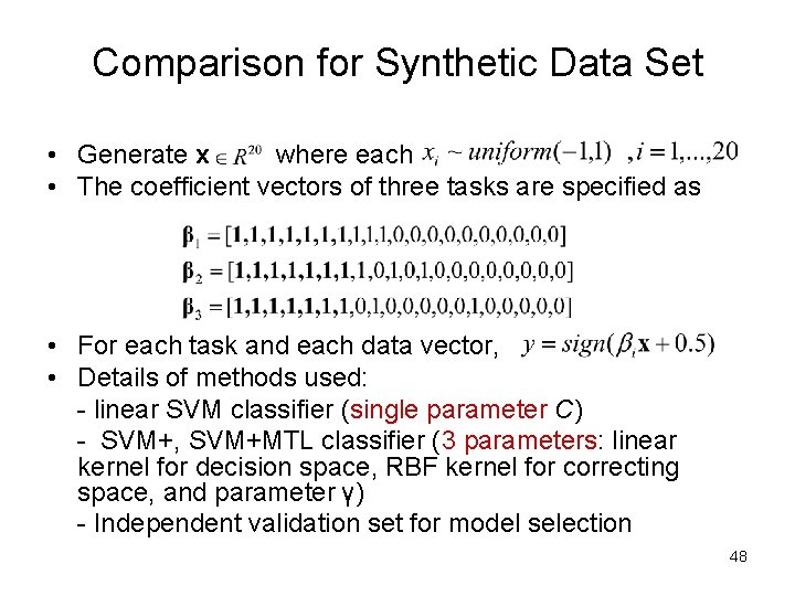
Comparison for Synthetic Data Set • Generate x where each • The coefficient vectors of three tasks are specified as • For each task and each data vector, • Details of methods used: - linear SVM classifier (single parameter C) - SVM+, SVM+MTL classifier (3 parameters: linear kernel for decision space, RBF kernel for correcting space, and parameter γ) - Independent validation set for model selection 48

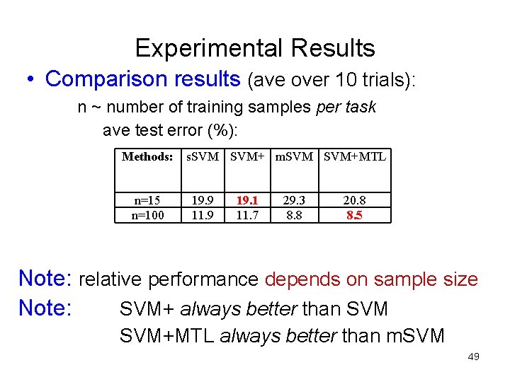
Experimental Results • Comparison results (ave over 10 trials): n ~ number of training samples per task ave test error (%): Methods: n=15 n=100 s. SVM+ m. SVM+MTL 19. 9 11. 9 19. 1 11. 7 29. 3 8. 8 20. 8 8. 5 Note: relative performance depends on sample size Note: SVM+ always better than SVM+MTL always better than m. SVM 49

OUTLINE • • • Motivation for non-standard approaches Alternative Learning Settings Summary: Advantages/limitations of nonstandard settings 50

Advantages+limitations of nonstandard settings • Advantages - make common sense - follow methodological framework (VC-theory) - yield better generalization (but not always) • Limitations - need to formalize application requirements need to understand application domain - generally more complex learning formulations - more difficult model selection - few known empirical comparisons (to date) • SVM+ is a promising new technology for hard problems 51

References and Resources • • • Vapnik, V. Estimation of Dependencies Based on Empirical Data. Empirical Inference Science: Afterword of 2006, Springer, 2006 Cherkassky, V. and F. Mulier, Learning from Data, second edition, Wiley, 2007 Chapelle, O. , Schölkopf, B. , and A. Zien, Eds. , Semi-Supervised Learning, MIT Press, 2006 Cherkassky, V. and Y. Ma, Introduction to Predictive learning, Springer, 2011 (to appear) Hastie, T. , R. Tibshirani and J. Friedman, The Elements of Statistical Learning. Data Mining, Inference and Prediction, New York: Springer, 2001 Schölkopf, B. and A. Smola, Learning with Kernels. MIT Press, 2002. Public-domain SVM software • • Main web page link http: //www. kernel-machines. org LIBSVM software library http: //www. csie. ntu. edu. tw/~cjlin/libsvm/ SVM-Light software library http: //svmlight. joachims. org/ Non-standard SVM-based methodologies: Universum, SVM+, MTL http: //www. ece. umn. edu/users/cherkass/predictive_learning/ 52