Part 3 SVM Practical Issues and Application Studies

Part 3: SVM Practical Issues and Application Studies Vladimir Cherkassky University of Minnesota cherk 001@umn. edu Presented at Tech Tune Ups, ECE Dept, June 1, 2011 Electrical and Computer Engineering 1

OUTLINE • • • Practical issues for SVM classifiers Univariate histograms of projections SVM model selection Application studies Summary 2

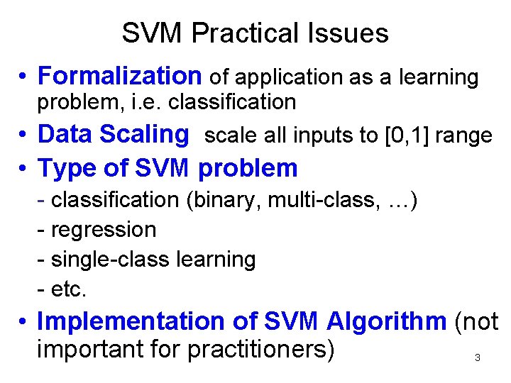
SVM Practical Issues • Formalization of application as a learning problem, i. e. classification • Data Scaling scale all inputs to [0, 1] range • Type of SVM problem - classification (binary, multi-class, …) - regression - single-class learning - etc. • Implementation of SVM Algorithm (not important for practitioners) 3

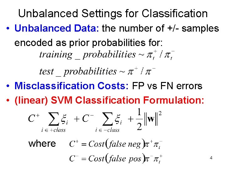
Unbalanced Settings for Classification • Unbalanced Data: the number of +/- samples encoded as prior probabilities for: • Misclassification Costs: FP vs FN errors • (linear) SVM Classification Formulation: where 4

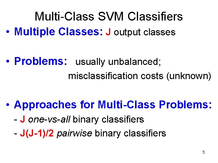
Multi-Class SVM Classifiers • Multiple Classes: J output classes • Problems: usually unbalanced; misclassification costs (unknown) • Approaches for Multi-Class Problems: - J one-vs-all binary classifiers - J(J-1)/2 pairwise binary classifiers 5

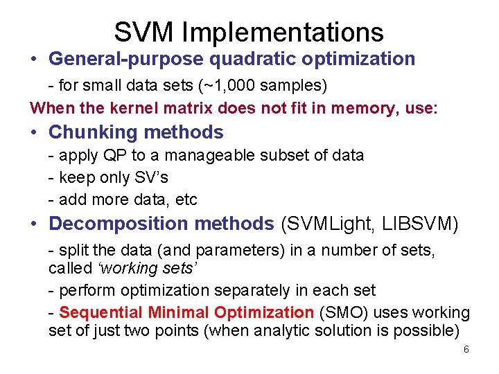
SVM Implementations • General-purpose quadratic optimization - for small data sets (~1, 000 samples) When the kernel matrix does not fit in memory, use: • Chunking methods - apply QP to a manageable subset of data - keep only SV’s - add more data, etc • Decomposition methods (SVMLight, LIBSVM) - split the data (and parameters) in a number of sets, called ‘working sets’ - perform optimization separately in each set - Sequential Minimal Optimization (SMO) uses working set of just two points (when analytic solution is possible) 6

OUTLINE • Practical issues for SVM classifiers • Univariate histograms for SVM classifiers • SVM model selection • Application studies • Summary 7

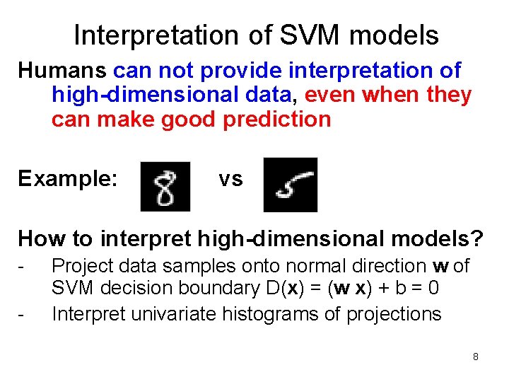
Interpretation of SVM models Humans can not provide interpretation of high-dimensional data, even when they can make good prediction Example: vs How to interpret high-dimensional models? - Project data samples onto normal direction w of SVM decision boundary D(x) = (w x) + b = 0 Interpret univariate histograms of projections 8

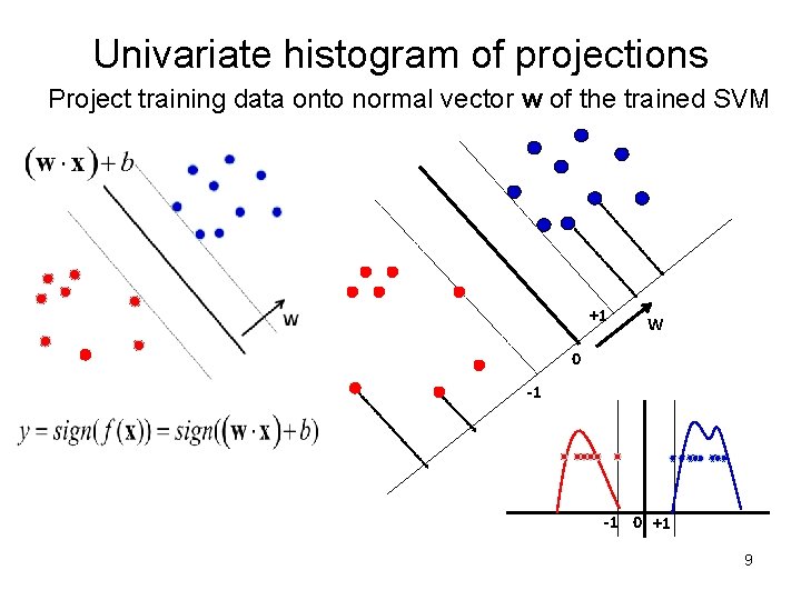
Univariate histogram of projections Project training data onto normal vector w of the trained SVM +1 W 0 -1 -1 0 +1 9

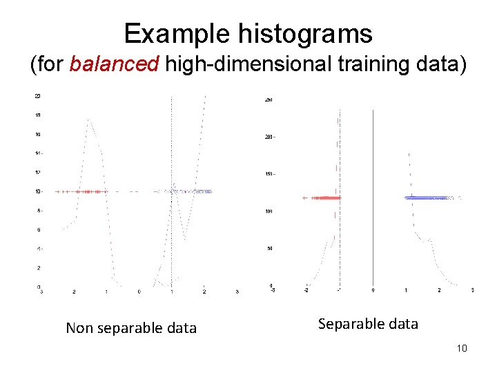
Example histograms (for balanced high-dimensional training data) Non separable data Separable data 10

OUTLINE • Practical issues for SVM classifiers • Univariate histograms of projections • SVM model selection - Model selection for classification - Model selection for regression • Application studies • Summary 11

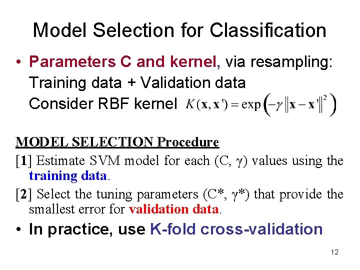
Model Selection for Classification • Parameters C and kernel, via resampling: Training data + Validation data Consider RBF kernel MODEL SELECTION Procedure [1] Estimate SVM model for each (C, γ) values using the training data. [2] Select the tuning parameters (C*, γ*) that provide the smallest error for validation data. • In practice, use K-fold cross-validation 12

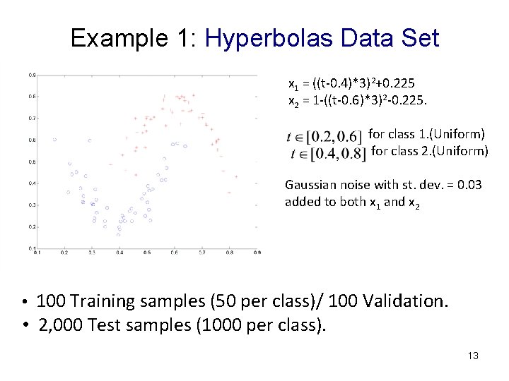
Example 1: Hyperbolas Data Set x 1 = ((t-0. 4)*3)2+0. 225 x 2 = 1 -((t-0. 6)*3)2 -0. 225. for class 1. (Uniform) for class 2. (Uniform) Gaussian noise with st. dev. = 0. 03 added to both x 1 and x 2 • 100 Training samples (50 per class)/ 100 Validation. • 2, 000 Test samples (1000 per class). 13

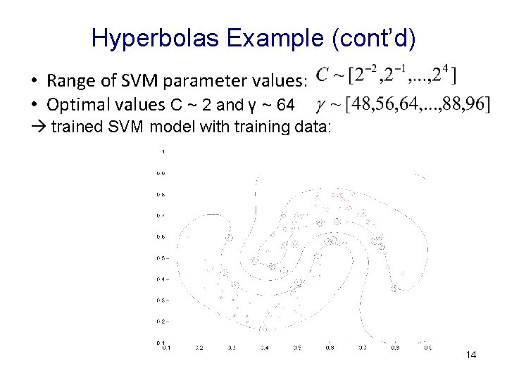
Hyperbolas Example (cont’d) • Range of SVM parameter values: • Optimal values C ~ 2 and γ ~ 64 trained SVM model with training data: 14

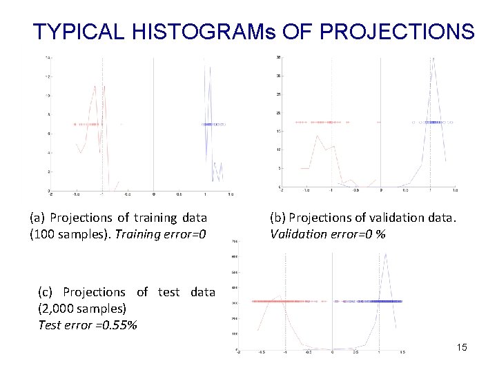
TYPICAL HISTOGRAMs OF PROJECTIONS (a) Projections of training data (100 samples). Training error=0 (b) Projections of validation data. Validation error=0 % (c) Projections of test data (2, 000 samples) Test error =0. 55% 15

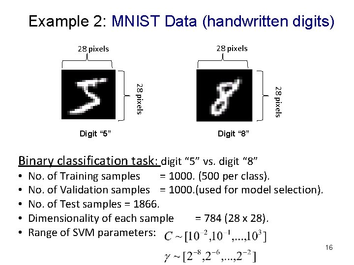
Example 2: MNIST Data (handwritten digits) 28 pixels Digit “ 5” Digit “ 8” Binary classification task: digit “ 5” vs. digit “ 8” • • • No. of Training samples = 1000. (500 per class). No. of Validation samples = 1000. (used for model selection). No. of Test samples = 1866. Dimensionality of each sample = 784 (28 x 28). Range of SVM parameters: 16

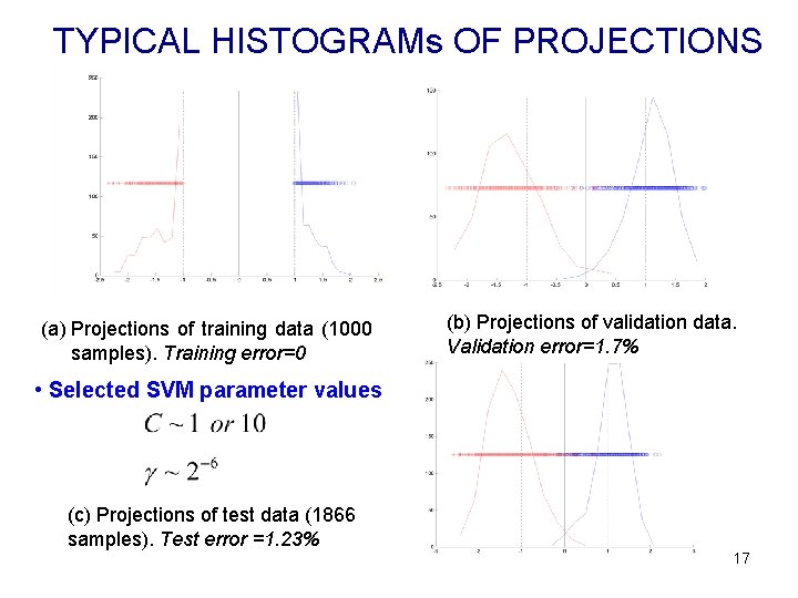
TYPICAL HISTOGRAMs OF PROJECTIONS (a) Projections of training data (1000 samples). Training error=0 (b) Projections of validation data. Validation error=1. 7% • Selected SVM parameter values (c) Projections of test data (1866 samples). Test error =1. 23% 17

Model Selection for HDLSS Data • High-Dim. Low Sample Size (HDLSS) - many applications: genomics, f. MRI… - sample size(~10’s)<<dimensionality (~1000) • Very Ill-Posed Problems • Issues for SVM classifiers (1) How to apply SVM classifiers to HDLSS? use linear SVM (2) How to perform model selection? 18

MNIST data under HDLSS scenario EXPERIMENTAL SETUP : - Binary classification digit “ 5” vs. digit “ 8” • No. of Training samples = 20 (10 per class). • No. of Validation samples = 20 ( for model selection). • No. of Test samples = 1866. • Dimensionality = 784 (28 x 28). • Model estimation method Linear SVM (single tuning parameter C) TWO MODEL SELECTION STRATEGIES for linear SVM: 1. Use independent validation set for tuning C 2. Set C to fixed large value providing maximum margin EXPERIMENTAL PROCEDURE: repeat comparison 10 times using 10 independent training/validation data sets 19

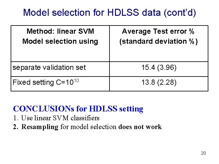
Model selection for HDLSS data (cont’d) Method: linear SVM Model selection using Average Test error % (standard deviation %) separate validation set 15. 4 (3. 96) Fixed setting C=1010 13. 8 (2. 28) CONCLUSIONs for HDLSS setting 1. Use linear SVM classifiers 2. Resampling for model selection does not work 20

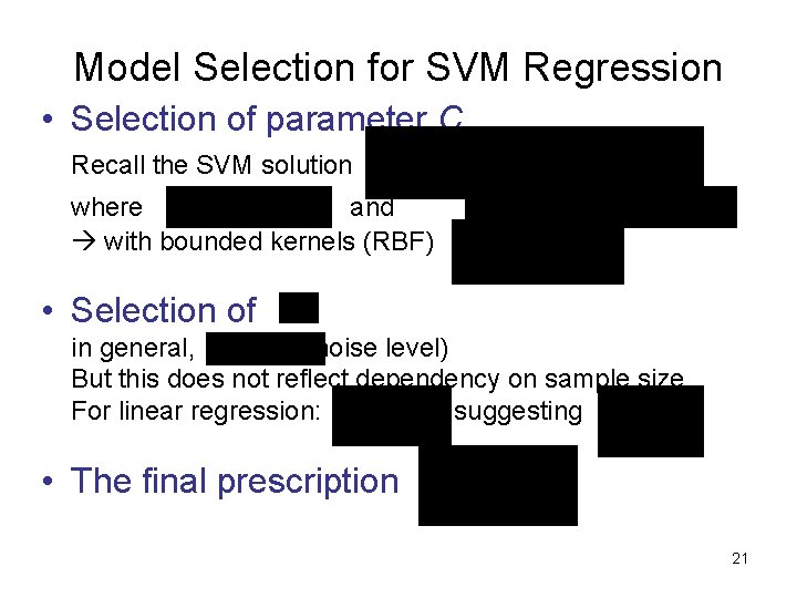
Model Selection for SVM Regression • Selection of parameter C Recall the SVM solution where and with bounded kernels (RBF) • Selection of in general, (noise level) But this does not reflect dependency on sample size For linear regression: suggesting • The final prescription 21

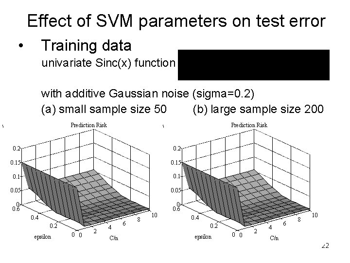
Effect of SVM parameters on test error • Training data univariate Sinc(x) function with additive Gaussian noise (sigma=0. 2) (a) small sample size 50 (b) large sample size 200 Prediction Risk 0. 2 0. 15 0. 1 0. 05 0 0 0. 6 0. 4 0. 2 epsilon 0 0 6 6 4 4 2 2 C/n 8 8 1010 0. 4 0. 2 epsilon 0 0 2 4 6 8 10 C/n 22

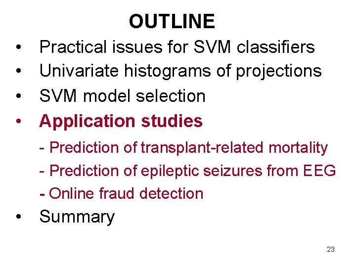
OUTLINE • • Practical issues for SVM classifiers Univariate histograms of projections SVM model selection Application studies - Prediction of transplant-related mortality - Prediction of epileptic seizures from EEG - Online fraud detection • Summary 23

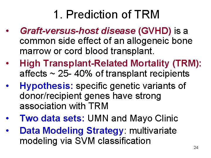
1. Prediction of TRM • • • Graft-versus-host disease (GVHD) is a common side effect of an allogeneic bone marrow or cord blood transplant. High Transplant-Related Mortality (TRM): affects ~ 25 - 40% of transplant recipients Hypothesis: specific genetic variants of donor/recipient genes have strong association with TRM Two data sets: UMN and Mayo Clinic Data Modeling Strategy: multivariate modeling via SVM classification 24

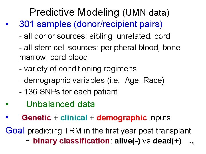
Predictive Modeling (UMN data) • 301 samples (donor/recipient pairs) - all donor sources: sibling, unrelated, cord - all stem cell sources: peripheral blood, bone marrow, cord blood - variety of conditioning regimens - demographic variables (i. e. , Age, Race) - 136 SNPs for each patient • Unbalanced data • Genetic + clinical + demographic inputs Goal predicting TRM in the first year post transplant ~ binary classification: alive(-) vs dead(+) 25

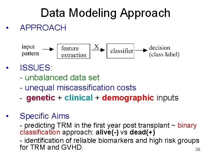
Data Modeling Approach • APPROACH • ISSUES: - unbalanced data set - unequal miscassification costs - genetic + clinical + demographic inputs • Specific Aims - predicting TRM in the first year post transplant ~ binary classification approach: alive(-) vs dead(+) - identification of reliable biomarkers and high risk groups for TRM and GVHD. 26

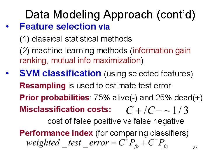
• Data Modeling Approach (cont’d) Feature selection via (1) classical statistical methods (2) machine learning methods (information gain ranking, mutual info maximization) • SVM classification (using selected features) Resampling is used to estimate test error Prior probabilities: 75% alive(-) and 25% dead(+) Misclassification costs: cost of false positive vs false negative Performance index (for comparing classifiers) 27

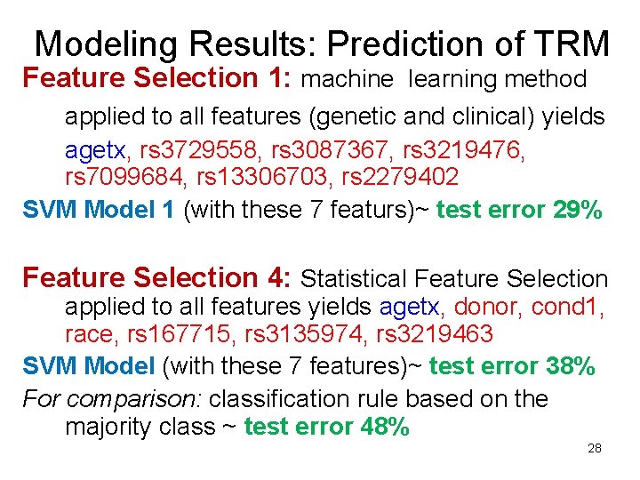
Modeling Results: Prediction of TRM Feature Selection 1: machine learning method applied to all features (genetic and clinical) yields agetx, rs 3729558, rs 3087367, rs 3219476, rs 7099684, rs 13306703, rs 2279402 SVM Model 1 (with these 7 featurs)~ test error 29% Feature Selection 4: Statistical Feature Selection applied to all features yields agetx, donor, cond 1, race, rs 167715, rs 3135974, rs 3219463 SVM Model (with these 7 features)~ test error 38% For comparison: classification rule based on the majority class ~ test error 48% 28

Modeling Results (cont’d) Feature Selection 3: machine learning method applied to genetic features only and then supplemented by clinical inputs provided by domain expert rs 3729558, rs 3219476, rs 13306703, rs 2279402, rs 3135974, rs 3138360, Rfc 5_13053, rs 3213391, rs 2066782, agetx, donor, cond 1 and race SVM Model 3(using these 13 inputs) ~ test error 29% Note: different SVM models 1 and 3 provide similar prediction error. Which one to interpret? 29

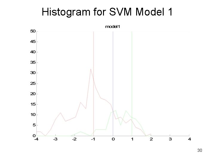
Histogram for SVM Model 1 30

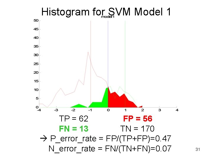
Histogram for SVM Model 1 TP = 62 FP = 56 FN = 13 TN = 170 P_error_rate = FP/(TP+FP)=0. 47 N_error_rate = FN/(TN+FN)=0. 07 31

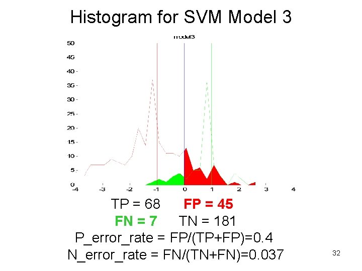
Histogram for SVM Model 3 TP = 68 FP = 45 FN = 7 TN = 181 P_error_rate = FP/(TP+FP)=0. 4 N_error_rate = FN/(TN+FN)=0. 037 32

Modeling Results: Mayo data set • • • Approach: apply the same modeling strategy Expectation: the same /similar generalization (because Mayo data set has the same statistical characteristics according to medical experts) Results: SVM model for Mayo data has poor prediction performance (not much better than random chance) • WHY? 33

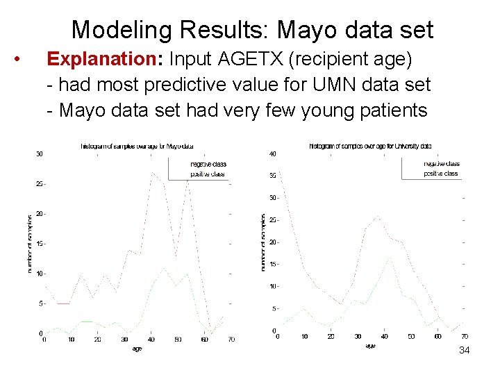
Modeling Results: Mayo data set • Explanation: Input AGETX (recipient age) - had most predictive value for UMN data set - Mayo data set had very few young patients 34

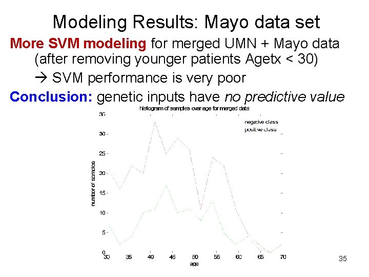
Modeling Results: Mayo data set More SVM modeling for merged UMN + Mayo data (after removing younger patients Agetx < 30) SVM performance is very poor Conclusion: genetic inputs have no predictive value 35

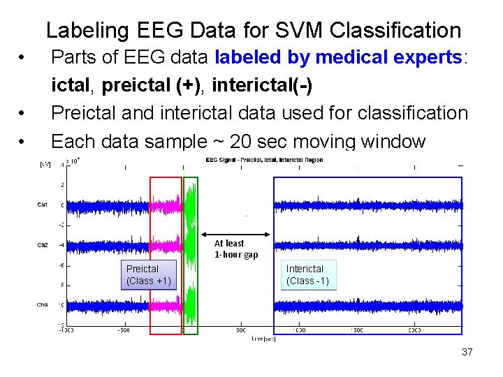
2. Prediction of Epileptic Seizures (Netoff, Park and Parhi 2009) • • • Objective: Patient-specific prediction of seizures (5 min ahead) from EEG signal (6 electrodes) Issues: performance metrics, unbalanced data, feature selection, sound methodology System implementation details: - features ~ power measured in 9 spectral bands for each electrode. Total 9 x 6 = 54 features - classifier ~ SVM with unequal costs - Freiburg data set 36

Labeling EEG Data for SVM Classification • • • Parts of EEG data labeled by medical experts: ictal, preictal (+), interictal(-) Preictal and interictal data used for classification Each data sample ~ 20 sec moving window At least 1 -hour gap Preictal (Class +1) Interictal (Class -1) 37

• Unbalanced data (patient 1): Total sample size: 9332 7. 7% positive (preictal), 92. 3% negative (interictal) 54 input features • Characterization of SVM method linear SVM misclassification costs Cost FN / Cost FP = 6 : 1 • Experimental procedure Double resampling for: - model selection - estimating test error (out-of-sample) 38

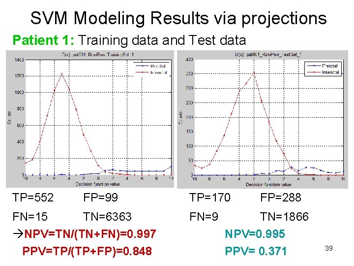
SVM Modeling Results via projections Patient 1: Training data and Test data TP=552 FP=99 FN=15 TN=6363 NPV=TN/(TN+FN)=0. 997 PPV=TP/(TP+FP)=0. 848 TP=170 FN=9 FP=288 TN=1866 NPV=0. 995 PPV= 0. 371 39

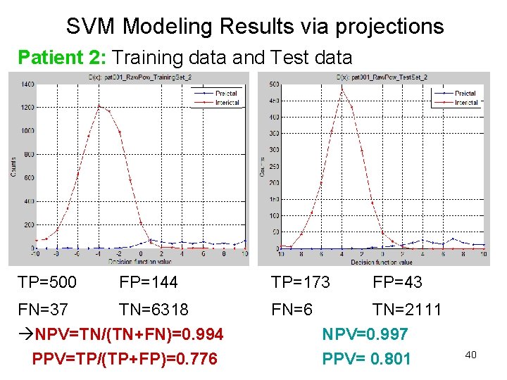
SVM Modeling Results via projections Patient 2: Training data and Test data TP=500 FP=144 FN=37 TN=6318 NPV=TN/(TN+FN)=0. 994 PPV=TP/(TP+FP)=0. 776 TP=173 FN=6 FP=43 TN=2111 NPV=0. 997 PPV= 0. 801 40

3. Online Fraud Detection (D. Chetty 2003) • • • Background on fraud detection On-line transaction processing Anti-Fraud strategies Learning problem set-up Modeling results 41

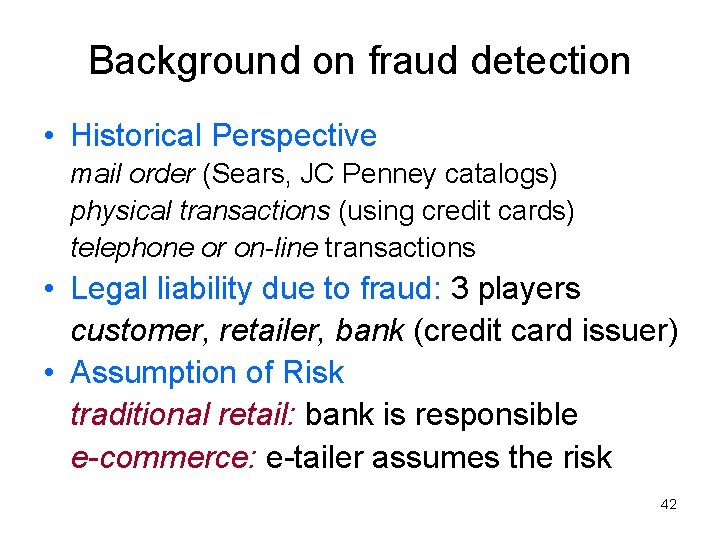
Background on fraud detection • Historical Perspective mail order (Sears, JC Penney catalogs) physical transactions (using credit cards) telephone or on-line transactions • Legal liability due to fraud: 3 players customer, retailer, bank (credit card issuer) • Assumption of Risk traditional retail: bank is responsible e-commerce: e-tailer assumes the risk 42

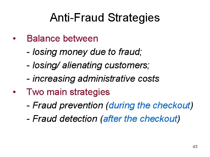
Anti-Fraud Strategies • • Balance between - losing money due to fraud; - losing/ alienating customers; - increasing administrative costs Two main strategies - Fraud prevention (during the checkout) - Fraud detection (after the checkout) 43

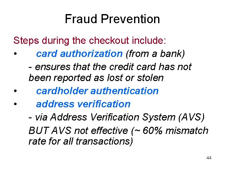
Fraud Prevention Steps during the checkout include: • card authorization (from a bank) - ensures that the credit card has not been reported as lost or stolen • cardholder authentication • address verification - via Address Verification System (AVS) BUT AVS not effective (~ 60% mismatch rate for all transactions) 44

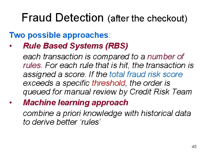
Fraud Detection (after the checkout) Two possible approaches: • Rule Based Systems (RBS) each transaction is compared to a number of rules. For each rule that is hit, the transaction is assigned a score. If the total fraud risk score exceeds a specific threshold, the order is queued for manual review by Credit Risk Team • Machine learning approach combine a priori knowledge with historical data to derive better ‘rules’ 45

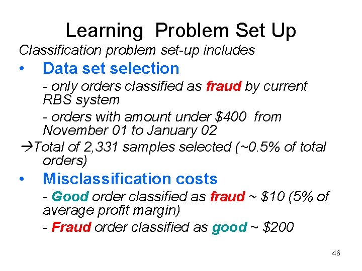
Learning Problem Set Up Classification problem set-up includes • Data set selection - only orders classified as fraud by current RBS system - orders with amount under $400 from November 01 to January 02 Total of 2, 331 samples selected (~0. 5% of total orders) • Misclassification costs - Good order classified as fraud ~ $10 (5% of average profit margin) - Fraud order classified as good ~ $200 46

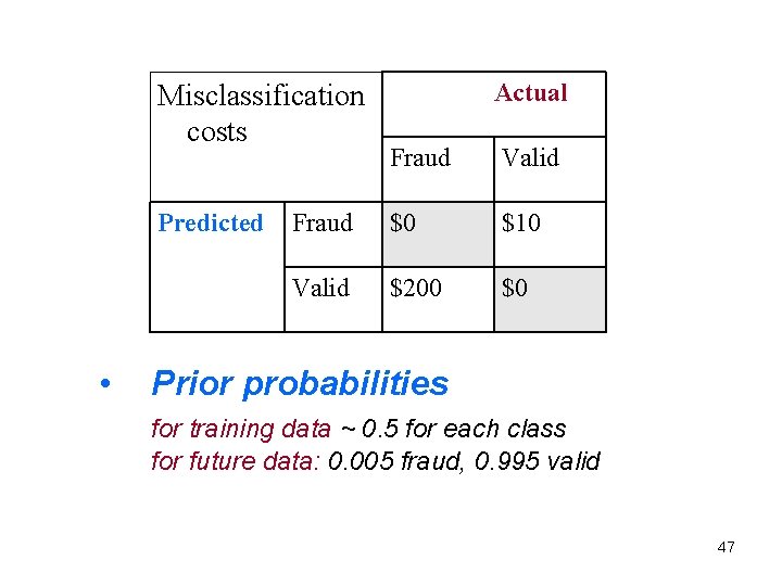
Misclassification costs Predicted • Actual Fraud Valid Fraud $0 $10 Valid $200 $0 Prior probabilities for training data ~ 0. 5 for each class for future data: 0. 005 fraud, 0. 995 valid 47

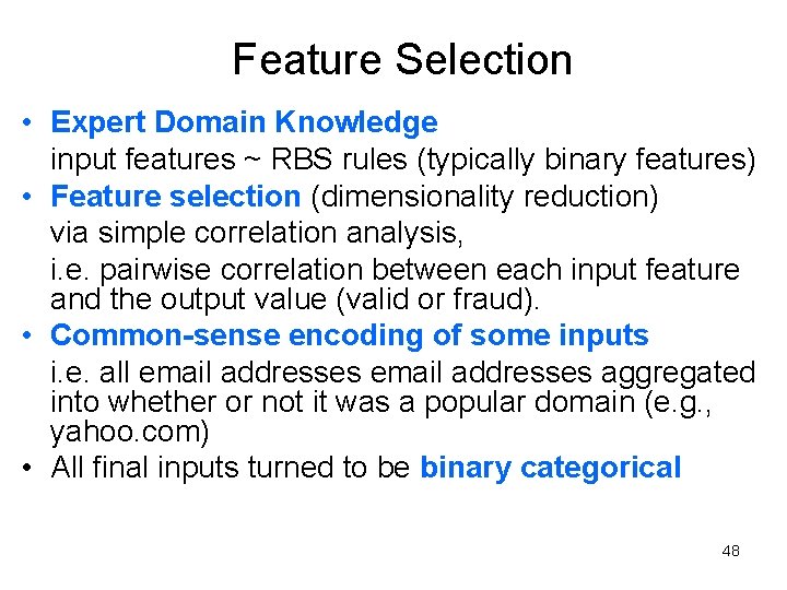
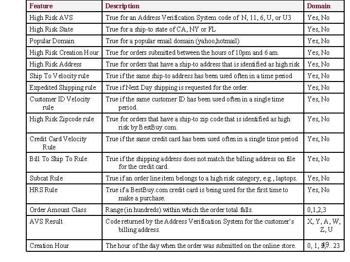
Feature Selection • Expert Domain Knowledge input features ~ RBS rules (typically binary features) • Feature selection (dimensionality reduction) via simple correlation analysis, i. e. pairwise correlation between each input feature and the output value (valid or fraud). • Common-sense encoding of some inputs i. e. all email addresses aggregated into whether or not it was a popular domain (e. g. , yahoo. com) • All final inputs turned to be binary categorical 48

Feature Description Domain High Risk AVS True for an Address Verification System code of N, 11, 6, U, or U 3 Yes, No High Risk State True for a ship-to state of CA, NY or FL Yes, No Popular Domain True for a popular email domain (yahoo, hotmail) Yes, No High Risk Creation Hour True for orders submitted between the hours of 10 pm and 6 am. Yes, No High Risk Address True for orders that have a ship-to address that is identified as high risk Yes, No Ship To Velocity rule True if the same ship-to address has been used often in a time period Yes, No Expedited Shipping rule True if Next Day shipping is requested for the order. Yes, No Customer ID Velocity rule True if the same customer ID has been used often in a single time period. Yes, No High Risk Zipcode rule True for orders that have a ship-to zip code that is identified as high risk by Best. Buy. com. Yes, No Credit Card Velocity Rule True if the same credit card has been used often in a single time period Yes, No Bill To Ship To Rule True if the shipping address does not match the billing address on file for the credit card. Yes, No Subcat Rule True if an order line item belongs to a high risk category, e. g. , laptops. Yes, No HRS Rule True if a Best. Buy. com credit card is being used for the first time to make a purchase. Yes, No Order Amount Class Range (in hundreds) within which the order total falls. 0, 1, 2, 3 AVS Result Code returned by the Address Verification System for the customer’s billing address. X, Y, A, W, Z, U Creation Hour The hour of the day when the order was submitted on the online store. 49 0, 1, 2, … 23

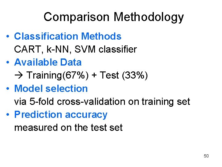
Comparison Methodology • Classification Methods CART, k-NN, SVM classifier • Available Data Training(67%) + Test (33%) • Model selection via 5 -fold cross-validation on training set • Prediction accuracy measured on the test set 50

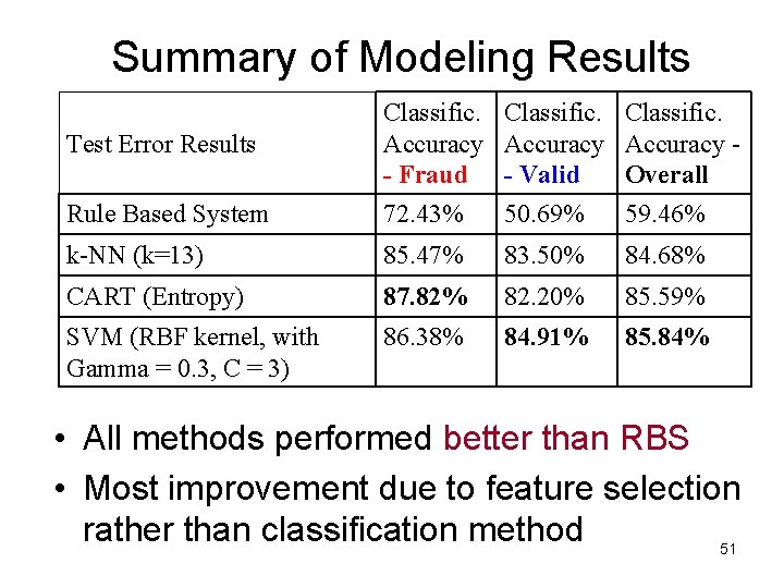
Summary of Modeling Results Rule Based System Classific. Accuracy - Fraud 72. 43% Classific. Accuracy - Valid 50. 69% Classific. Accuracy Overall 59. 46% k-NN (k=13) 85. 47% 83. 50% 84. 68% CART (Entropy) 87. 82% 82. 20% 85. 59% SVM (RBF kernel, with Gamma = 0. 3, C = 3) 86. 38% 84. 91% 85. 84% Test Error Results • All methods performed better than RBS • Most improvement due to feature selection rather than classification method 51

OUTLINE • Practical issues for SVM classifiers • Univariate histograms for SVM classifiers • SVM model selection • Application studies • Summary 52

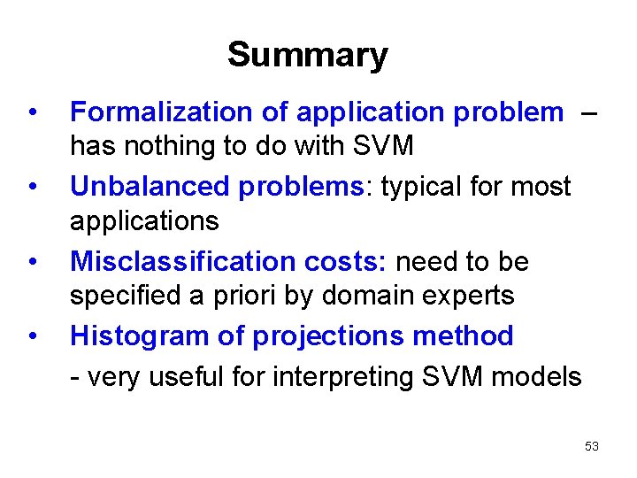
Summary • • Formalization of application problem – has nothing to do with SVM Unbalanced problems: typical for most applications Misclassification costs: need to be specified a priori by domain experts Histogram of projections method - very useful for interpreting SVM models 53