Part 3 Measurements and Models for Traffic Engineering

Part 3 Measurements and Models for Traffic Engineering

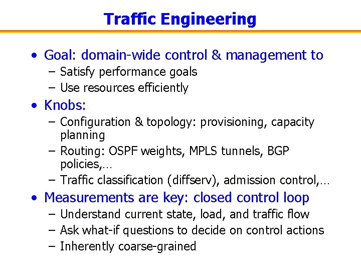
Traffic Engineering • Goal: domain-wide control & management to – Satisfy performance goals – Use resources efficiently • Knobs: – Configuration & topology: provisioning, capacity planning – Routing: OSPF weights, MPLS tunnels, BGP policies, … – Traffic classification (diffserv), admission control, … • Measurements are key: closed control loop – Understand current state, load, and traffic flow – Ask what-if questions to decide on control actions – Inherently coarse-grained

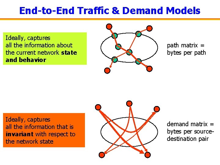
End-to-End Traffic & Demand Models Ideally, captures all the information about the current network state and behavior path matrix = bytes per path Ideally, captures all the information that is invariant with respect to the network state demand matrix = bytes per sourcedestination pair

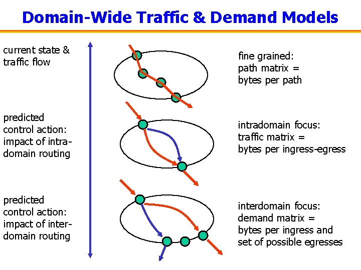
Domain-Wide Traffic & Demand Models current state & traffic flow predicted control action: impact of intradomain routing predicted control action: impact of interdomain routing fine grained: path matrix = bytes per path intradomain focus: traffic matrix = bytes per ingress-egress interdomain focus: demand matrix = bytes per ingress and set of possible egresses

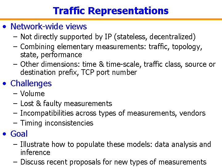
Traffic Representations • Network-wide views – Not directly supported by IP (stateless, decentralized) – Combining elementary measurements: traffic, topology, state, performance – Other dimensions: time & time-scale, traffic class, source or destination prefix, TCP port number • Challenges – – Volume Lost & faulty measurements Incompatibilities across types of measurements, vendors Timing inconsistencies • Goal – Illustrate how to populate these models: data analysis and inference – Discuss recent proposals for new types of measurements

Outline • Path matrix – Trajectory sampling – IP traceback • Traffic matrix – Network tomography • Demand matrix – Combining flow and routing data

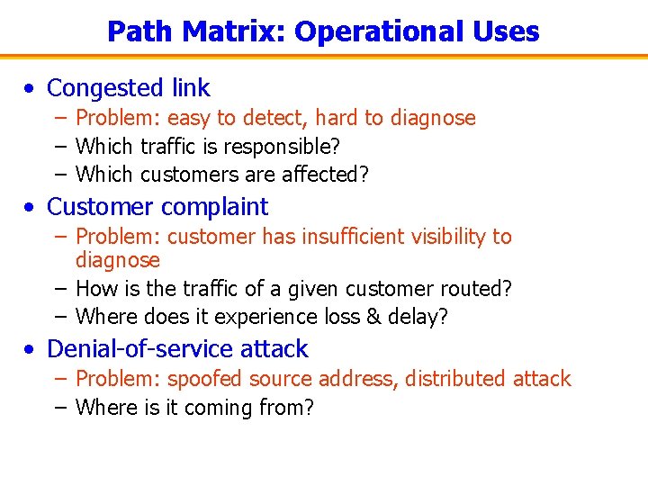
Path Matrix: Operational Uses • Congested link – Problem: easy to detect, hard to diagnose – Which traffic is responsible? – Which customers are affected? • Customer complaint – Problem: customer has insufficient visibility to diagnose – How is the traffic of a given customer routed? – Where does it experience loss & delay? • Denial-of-service attack – Problem: spoofed source address, distributed attack – Where is it coming from?

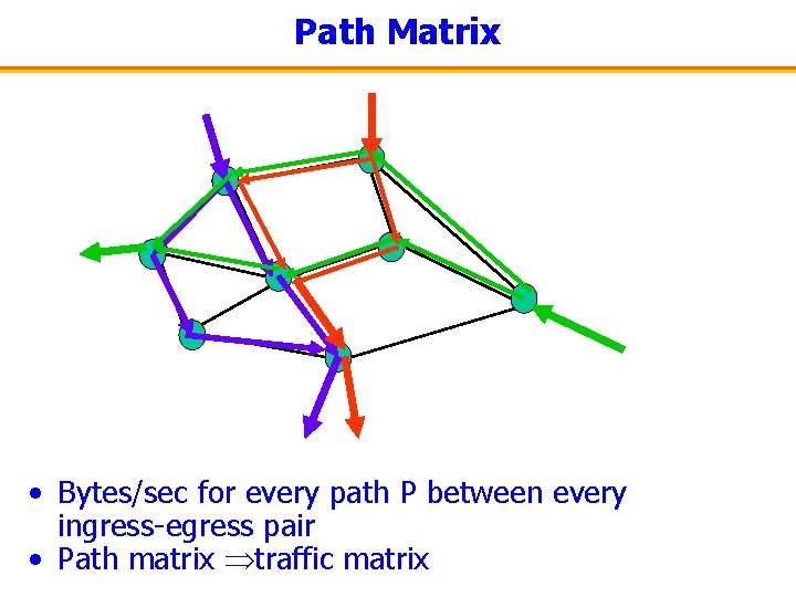
Path Matrix • Bytes/sec for every path P between every ingress-egress pair • Path matrix traffic matrix

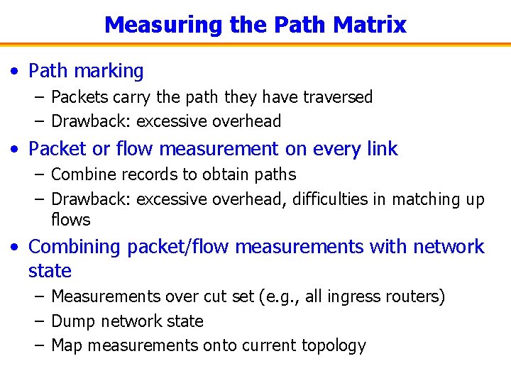
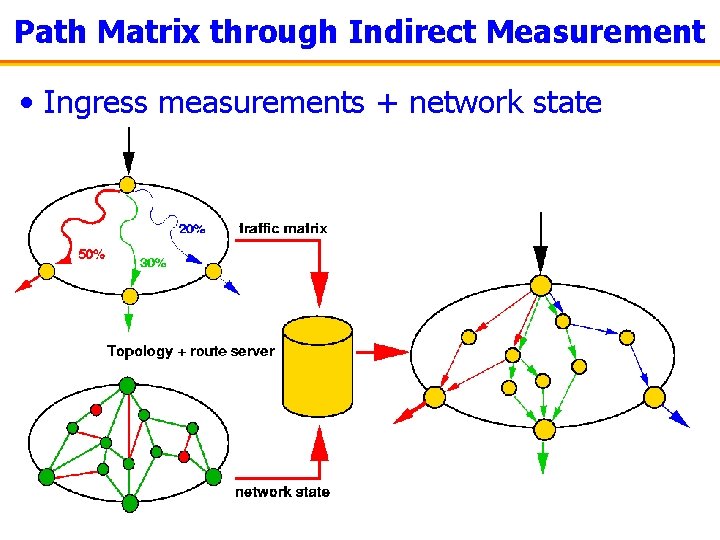
Measuring the Path Matrix • Path marking – Packets carry the path they have traversed – Drawback: excessive overhead • Packet or flow measurement on every link – Combine records to obtain paths – Drawback: excessive overhead, difficulties in matching up flows • Combining packet/flow measurements with network state – Measurements over cut set (e. g. , all ingress routers) – Dump network state – Map measurements onto current topology

Path Matrix through Indirect Measurement • Ingress measurements + network state

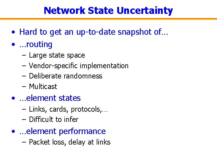
Network State Uncertainty • Hard to get an up-to-date snapshot of… • …routing – – Large state space Vendor-specific implementation Deliberate randomness Multicast • …element states – Links, cards, protocols, … – Difficult to infer • …element performance – Packet loss, delay at links

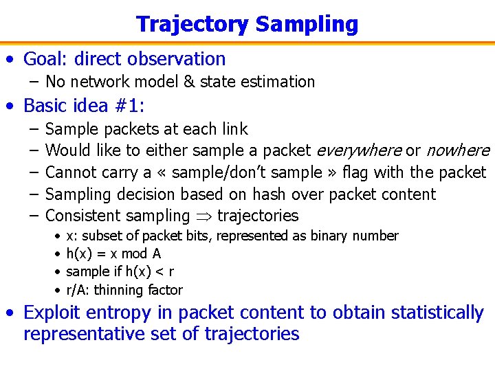
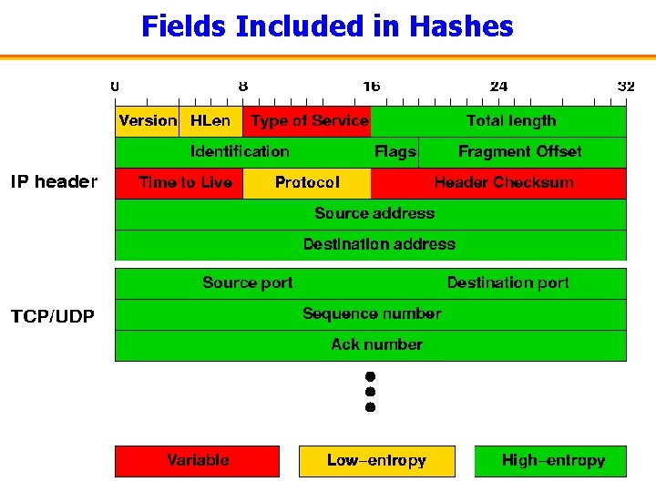
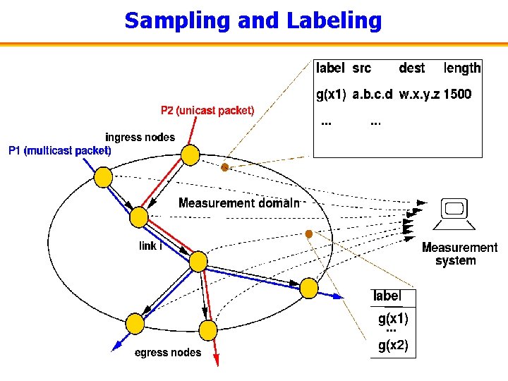
Trajectory Sampling • Goal: direct observation – No network model & state estimation • Basic idea #1: – – – Sample packets at each link Would like to either sample a packet everywhere or nowhere Cannot carry a « sample/don’t sample » flag with the packet Sampling decision based on hash over packet content Consistent sampling trajectories • • x: subset of packet bits, represented as binary number h(x) = x mod A sample if h(x) < r r/A: thinning factor • Exploit entropy in packet content to obtain statistically representative set of trajectories

Fields Included in Hashes

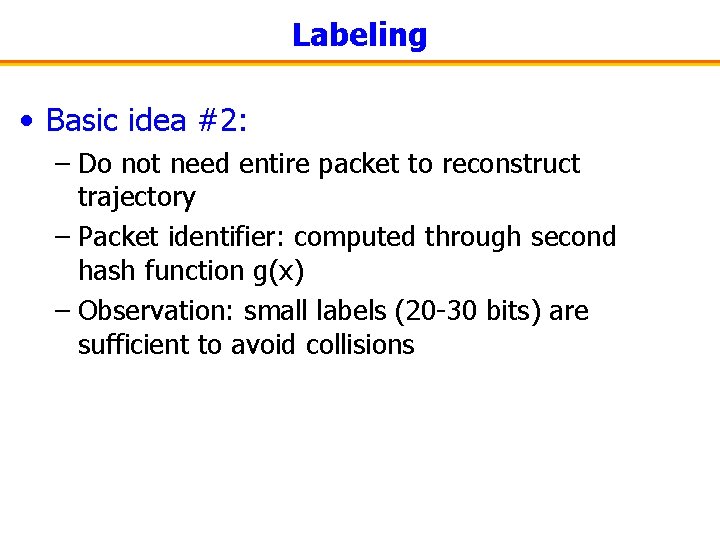
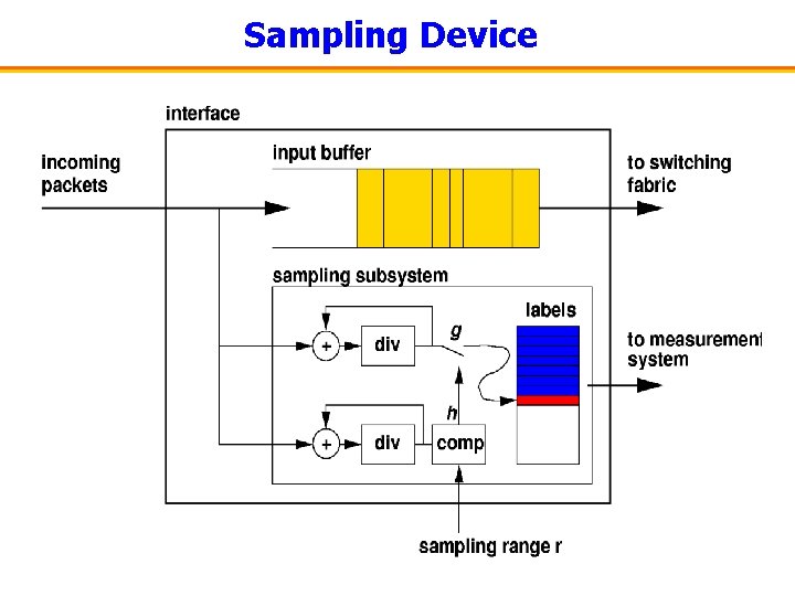
Labeling • Basic idea #2: – Do not need entire packet to reconstruct trajectory – Packet identifier: computed through second hash function g(x) – Observation: small labels (20 -30 bits) are sufficient to avoid collisions

Sampling and Labeling

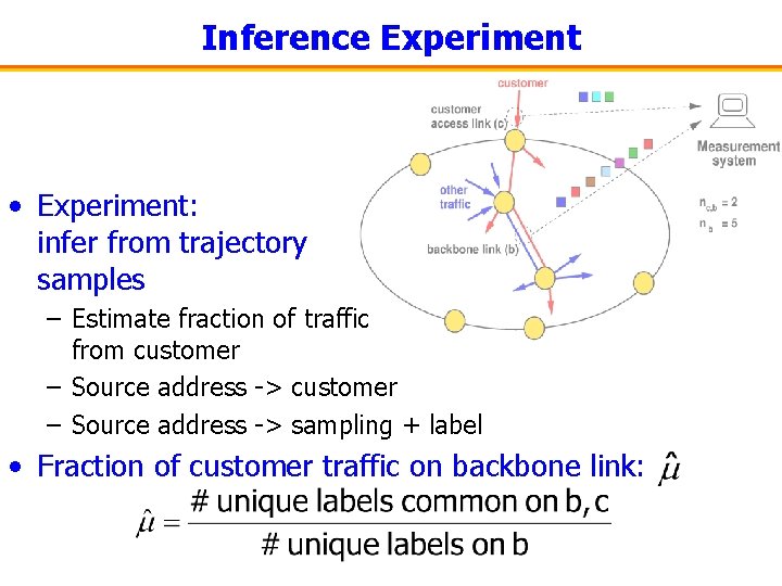
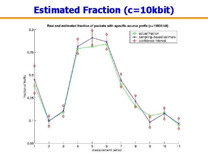
Inference Experiment • Experiment: infer from trajectory samples – Estimate fraction of traffic from customer – Source address -> sampling + label • Fraction of customer traffic on backbone link:

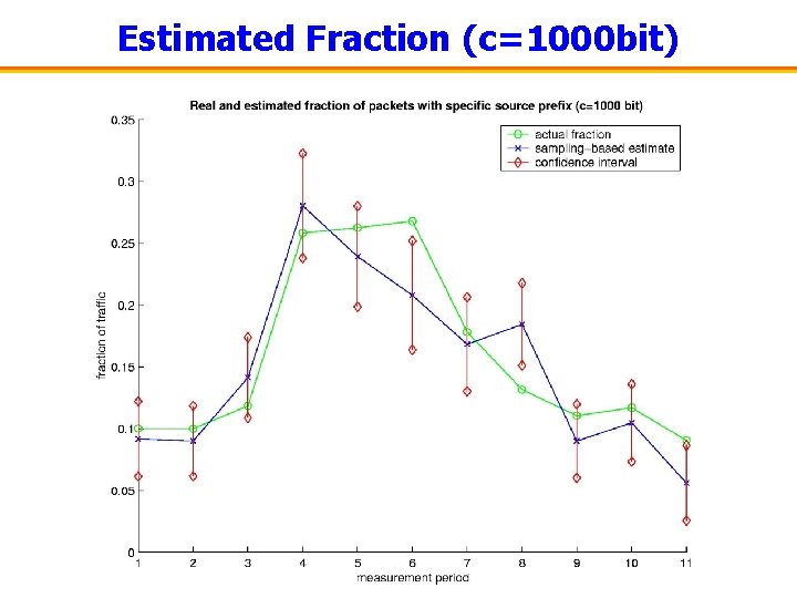
Estimated Fraction (c=1000 bit)

Estimated Fraction (c=10 kbit)

Sampling Device

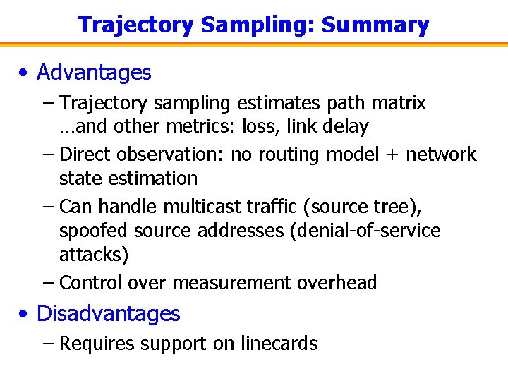
Trajectory Sampling: Summary • Advantages – Trajectory sampling estimates path matrix …and other metrics: loss, link delay – Direct observation: no routing model + network state estimation – Can handle multicast traffic (source tree), spoofed source addresses (denial-of-service attacks) – Control over measurement overhead • Disadvantages – Requires support on linecards

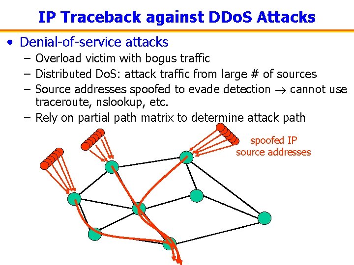
IP Traceback against DDo. S Attacks • Denial-of-service attacks – Overload victim with bogus traffic – Distributed Do. S: attack traffic from large # of sources – Source addresses spoofed to evade detection cannot use traceroute, nslookup, etc. – Rely on partial path matrix to determine attack path spoofed IP source addresses

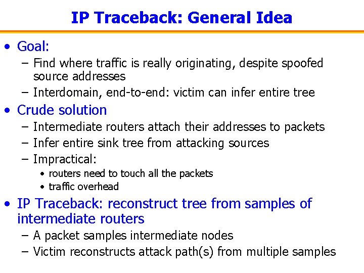
IP Traceback: General Idea • Goal: – Find where traffic is really originating, despite spoofed source addresses – Interdomain, end-to-end: victim can infer entire tree • Crude solution – Intermediate routers attach their addresses to packets – Infer entire sink tree from attacking sources – Impractical: • routers need to touch all the packets • traffic overhead • IP Traceback: reconstruct tree from samples of intermediate routers – A packet samples intermediate nodes – Victim reconstructs attack path(s) from multiple samples

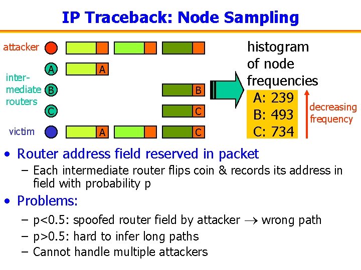
IP Traceback: Node Sampling attacker A intermediate B routers C victim A B C A C histogram of node frequencies A: 239 decreasing B: 493 frequency C: 734 • Router address field reserved in packet – Each intermediate router flips coin & records its address in field with probability p • Problems: – p<0. 5: spoofed router field by attacker wrong path – p>0. 5: hard to infer long paths – Cannot handle multiple attackers

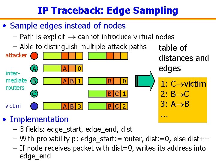
IP Traceback: Edge Sampling • Sample edges instead of nodes – Path is explicit cannot introduce virtual nodes – Able to distinguish multiple attack paths table of attacker distances and A A 0 edges intermediate B routers C A B 1 victim A B 3 B 0 B C 1 • Implementation B C 2 1: C victim 2: B C 3: A B. . . – 3 fields: edge_start, edge_end, dist – With probability p: edge_start: =router, dist: =0, else dist++ – If node receives packet with dist=0, writes its address into edge_end

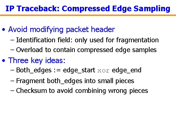
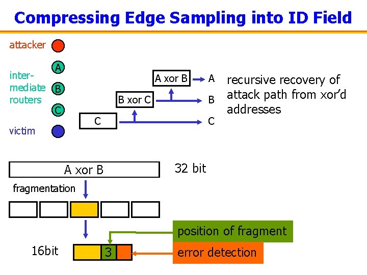
IP Traceback: Compressed Edge Sampling • Avoid modifying packet header – Identification field: only used for fragmentation – Overload to contain compressed edge samples • Three key ideas: – Both_edges : = edge_start xor edge_end – Fragment both_edges into small pieces – Checksum to avoid combining wrong pieces

Compressing Edge Sampling into ID Field attacker A intermediate B routers C A xor B B xor C B C victim A C recursive recovery of attack path from xor’d addresses 32 bit A xor B fragmentation position of fragment 16 bit 3 error detection

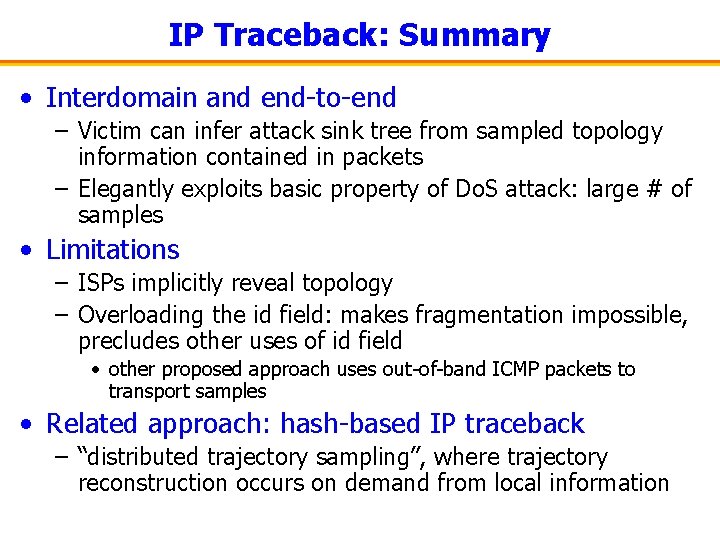
IP Traceback: Summary • Interdomain and end-to-end – Victim can infer attack sink tree from sampled topology information contained in packets – Elegantly exploits basic property of Do. S attack: large # of samples • Limitations – ISPs implicitly reveal topology – Overloading the id field: makes fragmentation impossible, precludes other uses of id field • other proposed approach uses out-of-band ICMP packets to transport samples • Related approach: hash-based IP traceback – “distributed trajectory sampling”, where trajectory reconstruction occurs on demand from local information

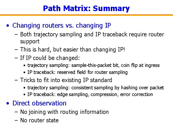
Path Matrix: Summary • Changing routers vs. changing IP – Both trajectory sampling and IP traceback require router support – This is hard, but easier than changing IP! – If IP could be changed: • trajectory sampling: sample-this-packet bit, coin flip at ingress • IP traceback: reserved field for router sampling – Tricks to fit into existing IP standard • trajectory sampling: consistent sampling by hashing over packet • IP traceback: edge sampling, compression, error correction • Direct observation – No joining with routing information – No router state

Outline • Path matrix – Trajectory sampling – IP traceback • Traffic matrix – Network tomography • Demand matrix – Combining flow and routing data

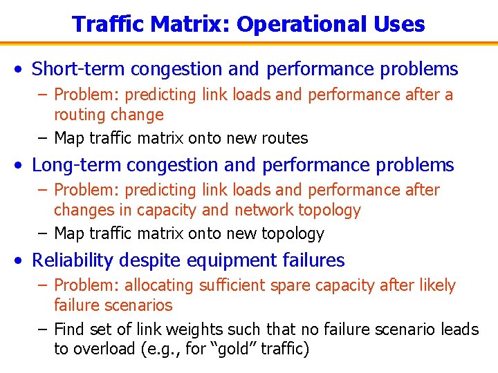
Traffic Matrix: Operational Uses • Short-term congestion and performance problems – Problem: predicting link loads and performance after a routing change – Map traffic matrix onto new routes • Long-term congestion and performance problems – Problem: predicting link loads and performance after changes in capacity and network topology – Map traffic matrix onto new topology • Reliability despite equipment failures – Problem: allocating sufficient spare capacity after likely failure scenarios – Find set of link weights such that no failure scenario leads to overload (e. g. , for “gold” traffic)

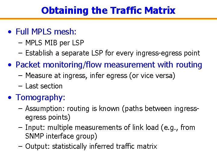
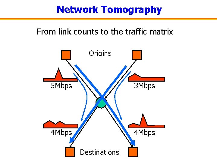
Obtaining the Traffic Matrix • Full MPLS mesh: – MPLS MIB per LSP – Establish a separate LSP for every ingress-egress point • Packet monitoring/flow measurement with routing – Measure at ingress, infer egress (or vice versa) – Last section • Tomography: – Assumption: routing is known (paths between ingressegress points) – Input: multiple measurements of link load (e. g. , from SNMP interface group) – Output: statistically inferred traffic matrix

Network Tomography From link counts to the traffic matrix Origins 5 Mbps 3 Mbps 4 Mbps Destinations

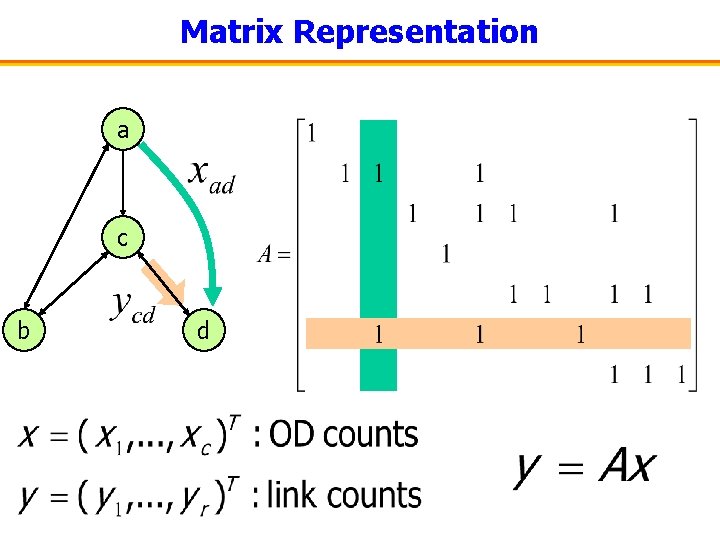
Matrix Representation a c b d

Single Observation is Insufficient • Linear system is underdetermined – Number of links – Number of OD pairs – Dimension of solution sub-space at least • Multiple observations are needed – Stochastic model to bind them

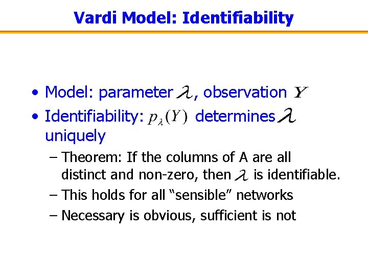
Network Tomography • [Y. Vardi, Network Tomography, JASA, March 1996] • Inspired by road traffic networks, medical tomography • Assumptions: – OD counts independent & identically distributed (i. i. d. ) – K independent observations

Vardi Model: Identifiability • Model: parameter • Identifiability: uniquely , observation determines – Theorem: If the columns of A are all distinct and non-zero, then is identifiable. – This holds for all “sensible” networks – Necessary is obvious, sufficient is not

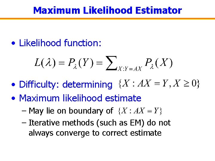
Maximum Likelihood Estimator • Likelihood function: • Difficulty: determining • Maximum likelihood estimate – May lie on boundary of – Iterative methods (such as EM) do not always converge to correct estimate

Estimator Based on Method of Moments • Gaussian approximation of sample mean • Match mean+covariance of model to sample mean+covariance of observation • Mean: • Cross-covariance:

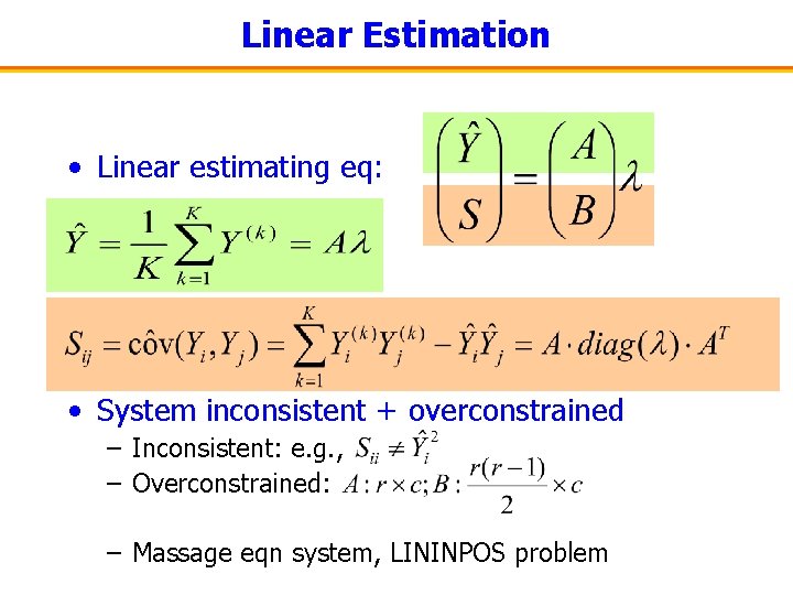
Linear Estimation • Linear estimating eq: • System inconsistent + overconstrained – Inconsistent: e. g. , – Overconstrained: – Massage eqn system, LININPOS problem

How Well does it Work? • Experiment [Vardi]: – K=100 • Limitations: – Poisson traffic – Small network a c b d

Further Papers on Tomography • [J. Cao et al. , Time-Varying Network Tomography, JASA, Dec 2000] – Gaussian traffic model, mean-variance scaling • [Tebaldi & West, Bayesian Inference on Network Traffic…, JASA, June 1998] – Single observation, Bayesian prior • [J. Cao et al. , Scalable Method…, submitted, 2001] – Heuristics for efficient computation

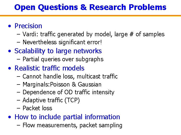
Open Questions & Research Problems • Precision – Vardi: traffic generated by model, large # of samples – Nevertheless significant error! • Scalability to large networks – Partial queries over subgraphs • Realistic traffic models – – – Cannot handle loss, multicast traffic Marginals: Poisson & Gaussian Dependence of OD traffic intensity Adaptive traffic (TCP) Packet loss • How to include partial information – Flow measurements, packet sampling

Outline • Path matrix – Trajectory sampling – IP traceback • Traffic matrix – Network tomography • Demand matrix – Combining flow and routing data

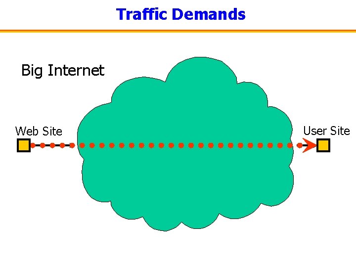
Traffic Demands Big Internet Web Site User Site

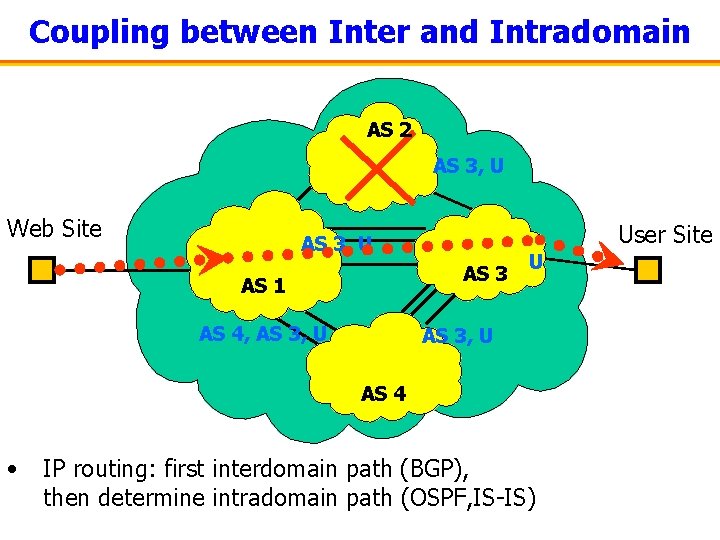
Coupling between Inter and Intradomain AS 2 AS 3, U Web Site User Site AS 3, U AS 3 AS 1 AS 4, AS 3, U U AS 3, U AS 4 • IP routing: first interdomain path (BGP), then determine intradomain path (OSPF, IS-IS)

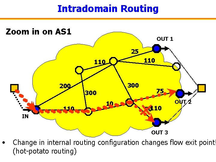
Intradomain Routing Zoom in on AS 1 OUT 1 25 110 200 110 300 10 75 50110 OUT 2 IN OUT 3 • Change in internal routing configuration changes flow exit point! (hot-potato routing)

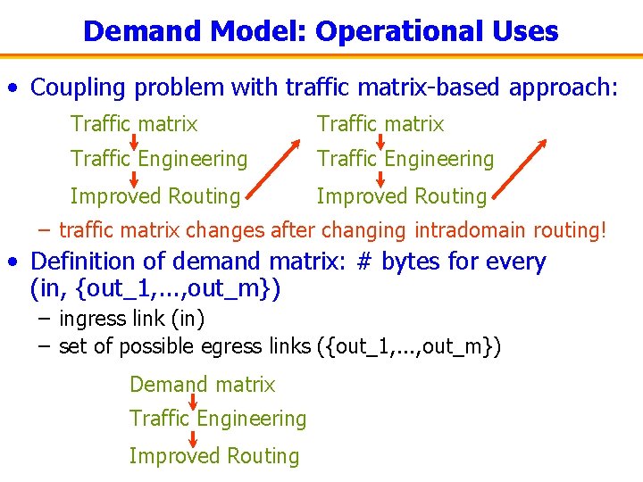
Demand Model: Operational Uses • Coupling problem with traffic matrix-based approach: Traffic matrix Traffic Engineering Improved Routing – traffic matrix changes after changing intradomain routing! • Definition of demand matrix: # bytes for every (in, {out_1, . . . , out_m}) – ingress link (in) – set of possible egress links ({out_1, . . . , out_m}) Demand matrix Traffic Engineering Improved Routing

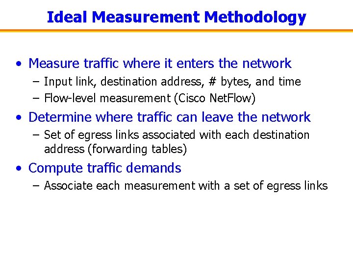
Ideal Measurement Methodology • Measure traffic where it enters the network – Input link, destination address, # bytes, and time – Flow-level measurement (Cisco Net. Flow) • Determine where traffic can leave the network – Set of egress links associated with each destination address (forwarding tables) • Compute traffic demands – Associate each measurement with a set of egress links

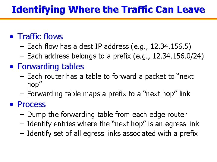
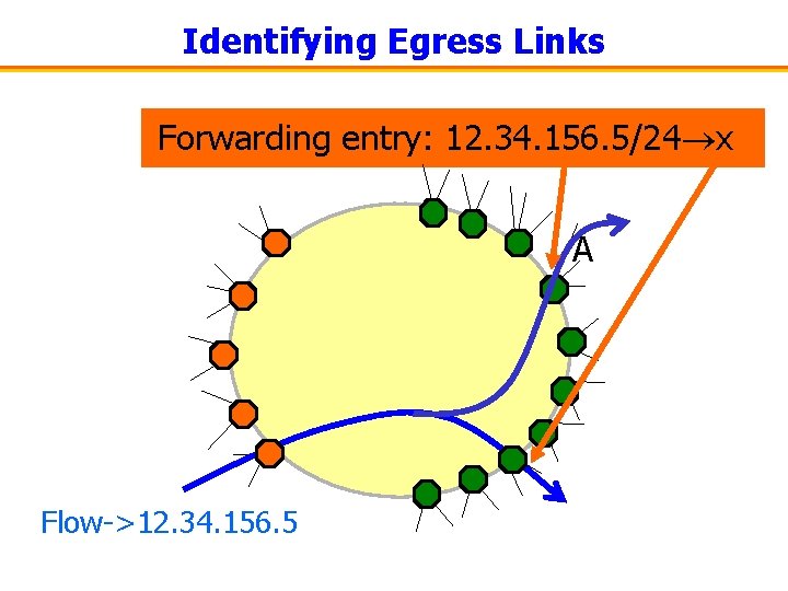
Identifying Where the Traffic Can Leave • Traffic flows – Each flow has a dest IP address (e. g. , 12. 34. 156. 5) – Each address belongs to a prefix (e. g. , 12. 34. 156. 0/24) • Forwarding tables – Each router has a table to forward a packet to “next hop” – Forwarding table maps a prefix to a “next hop” link • Process – Dump the forwarding table from each edge router – Identify entries where the “next hop” is an egress link – Identify set of all egress links associated with a prefix

Identifying Egress Links Forwarding entry: 12. 34. 156. 5/24 x A Flow->12. 34. 156. 5

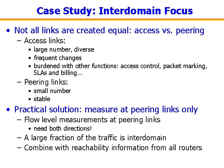
Case Study: Interdomain Focus • Not all links are created equal: access vs. peering – Access links: • large number, diverse • frequent changes • burdened with other functions: access control, packet marking, SLAs and billing. . . – Peering links: • small number • stable • Practical solution: measure at peering links only – Flow level measurements at peering links • need both directions! – A large fraction of the traffic is interdomain – Combine with reachability information from all routers

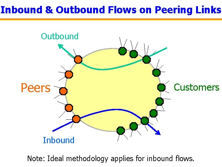
Inbound & Outbound Flows on Peering Links Outbound Peers Customers Inbound Note: Ideal methodology applies for inbound flows.

Flows Leaving at Peer Links • Transit traffic – Problem: avoid double-counting – Either in and out at same or at different routers – Idea: use source address to check if flow originates at customer • trustworthy because of ingress filtering of customer traffic • Outbound traffic – Flow measured only as it leaves the network – Keep flow record if source address matches a customer – Identify ingress link(s) that could have sent the traffic

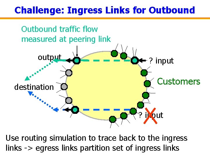
Challenge: Ingress Links for Outbound traffic flow measured at peering link output destination ? input Customers ? input Use routing simulation to trace back to the ingress links -> egress links partition set of ingress links

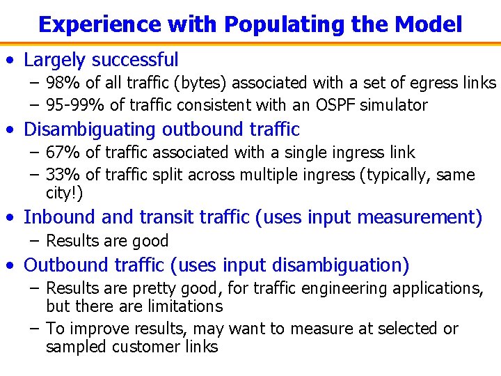
Experience with Populating the Model • Largely successful – 98% of all traffic (bytes) associated with a set of egress links – 95 -99% of traffic consistent with an OSPF simulator • Disambiguating outbound traffic – 67% of traffic associated with a single ingress link – 33% of traffic split across multiple ingress (typically, same city!) • Inbound and transit traffic (uses input measurement) – Results are good • Outbound traffic (uses input disambiguation) – Results are pretty good, for traffic engineering applications, but there are limitations – To improve results, may want to measure at selected or sampled customer links

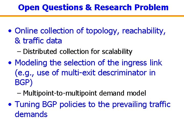
Open Questions & Research Problem • Online collection of topology, reachability, & traffic data – Distributed collection for scalability • Modeling the selection of the ingress link (e. g. , use of multi-exit descriminator in BGP) – Multipoint-to-multipoint demand model • Tuning BGP policies to the prevailing traffic demands

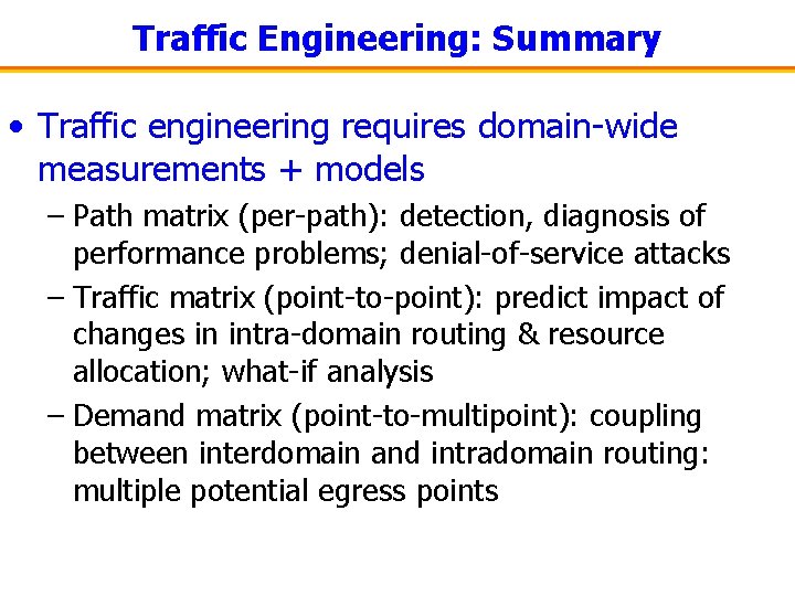
Traffic Engineering: Summary • Traffic engineering requires domain-wide measurements + models – Path matrix (per-path): detection, diagnosis of performance problems; denial-of-service attacks – Traffic matrix (point-to-point): predict impact of changes in intra-domain routing & resource allocation; what-if analysis – Demand matrix (point-to-multipoint): coupling between interdomain and intradomain routing: multiple potential egress points

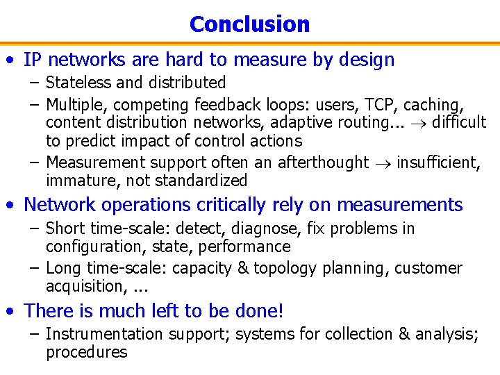
Conclusion • IP networks are hard to measure by design – Stateless and distributed – Multiple, competing feedback loops: users, TCP, caching, content distribution networks, adaptive routing. . . difficult to predict impact of control actions – Measurement support often an afterthought insufficient, immature, not standardized • Network operations critically rely on measurements – Short time-scale: detect, diagnose, fix problems in configuration, state, performance – Long time-scale: capacity & topology planning, customer acquisition, . . . • There is much left to be done! – Instrumentation support; systems for collection & analysis; procedures