Part 3 Linear Programming 3 2 Algorithm General

Part 3. Linear Programming 3. 2 Algorithm

General Formulation Convex function Convex region

Example

Profit Amount of product p Amount of crude c

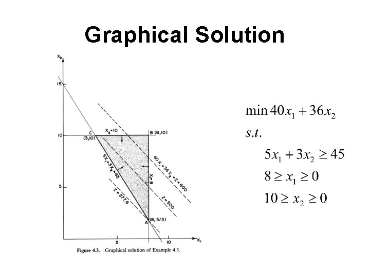
Graphical Solution

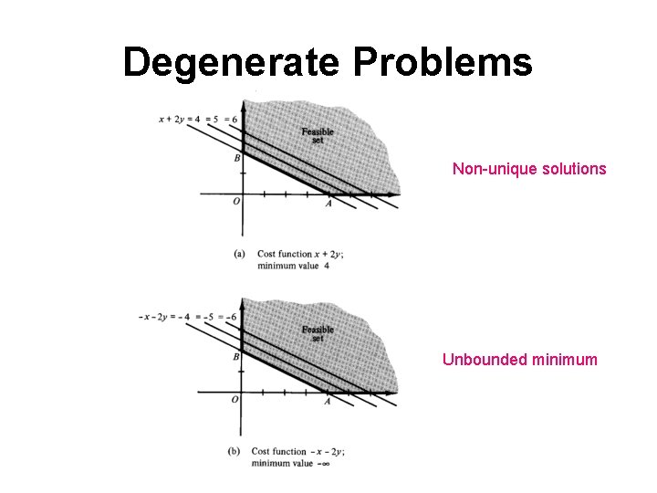
Degenerate Problems Non-unique solutions Unbounded minimum

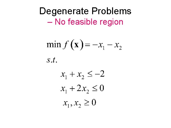
Degenerate Problems – No feasible region

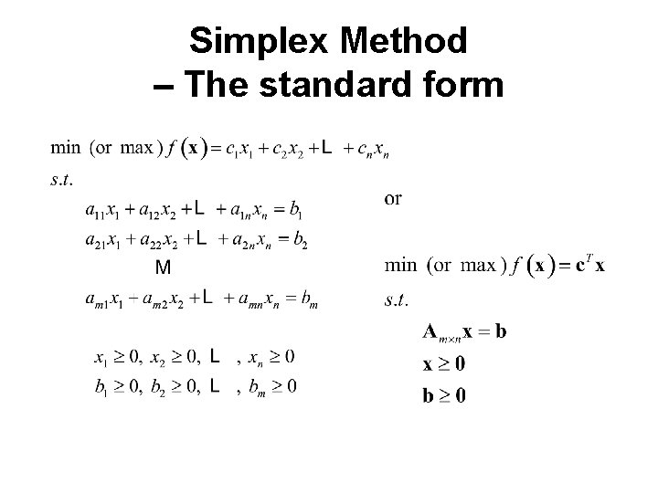
Simplex Method – The standard form

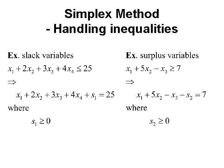
Simplex Method - Handling inequalities

Simplex Method - Handling unrestricted variables

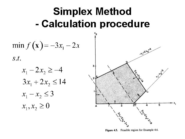
Simplex Method - Calculation procedure

Calculation Procedure - Step 0

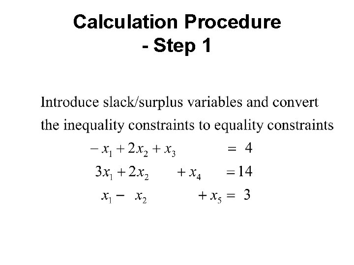
Calculation Procedure - Step 1

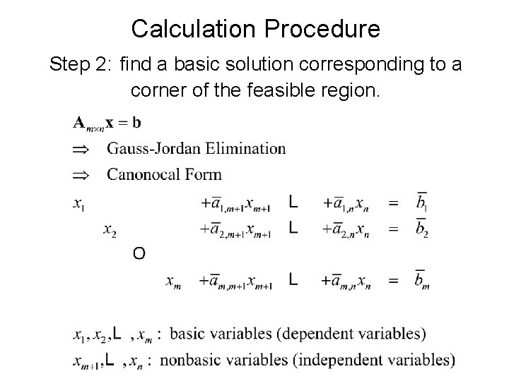
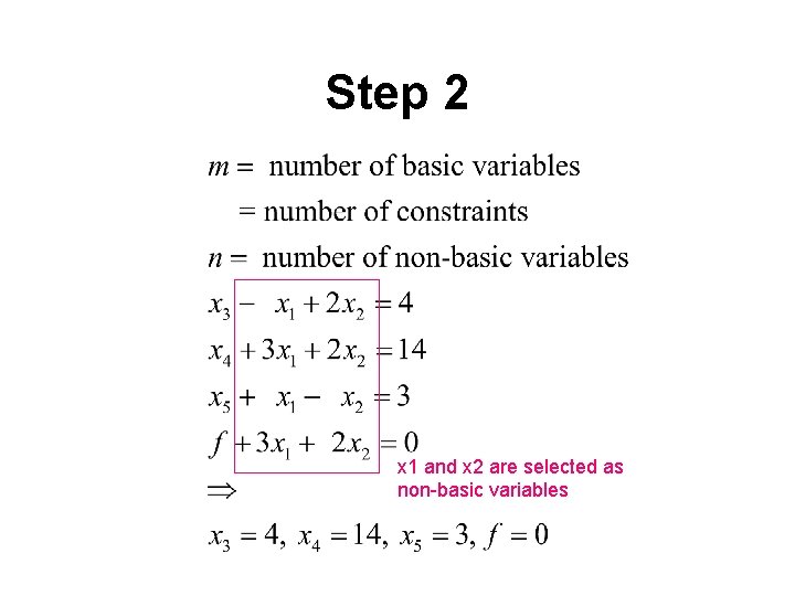
Calculation Procedure Step 2: find a basic solution corresponding to a corner of the feasible region.

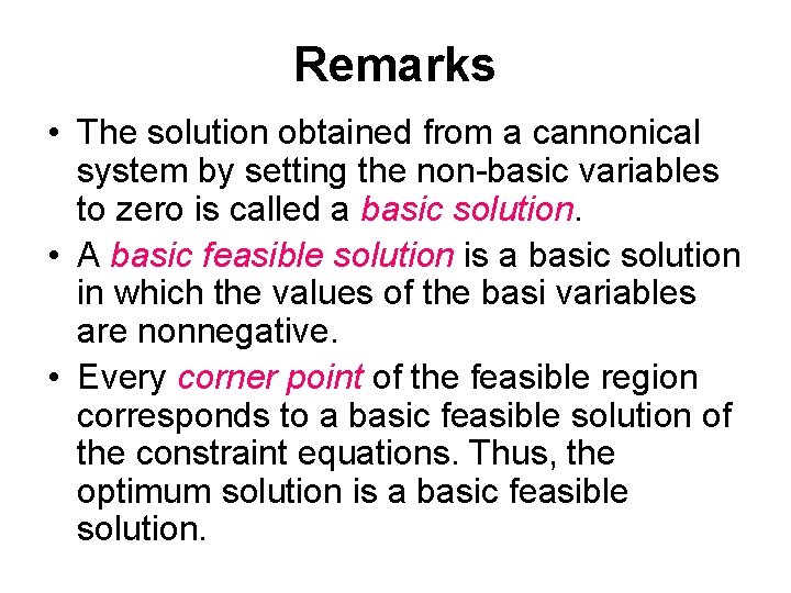
Remarks • The solution obtained from a cannonical system by setting the non-basic variables to zero is called a basic solution. • A basic feasible solution is a basic solution in which the values of the basi variables are nonnegative. • Every corner point of the feasible region corresponds to a basic feasible solution of the constraint equations. Thus, the optimum solution is a basic feasible solution.

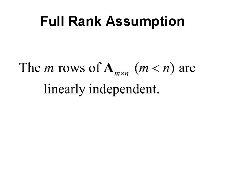
Full Rank Assumption

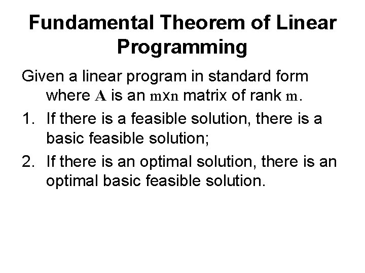
Fundamental Theorem of Linear Programming Given a linear program in standard form where A is an mxn matrix of rank m. 1. If there is a feasible solution, there is a basic feasible solution; 2. If there is an optimal solution, there is an optimal basic feasible solution.

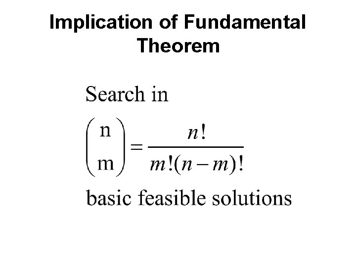
Implication of Fundamental Theorem

Extreme Point

Theorem (Equivalence of extreme points and basic solutions)

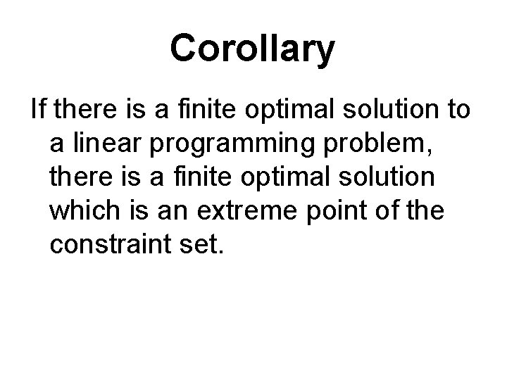
Corollary If there is a finite optimal solution to a linear programming problem, there is a finite optimal solution which is an extreme point of the constraint set.

Step 2 x 1 and x 2 are selected as non-basic variables

Step 3: select new basic and non -basic variables new basic variable

Which one of x 3, x 4, x 5 should be selected as the new non-basic variables?

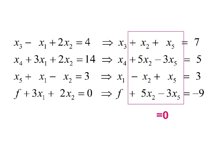
Step 4: Transformation of the Equations

=0

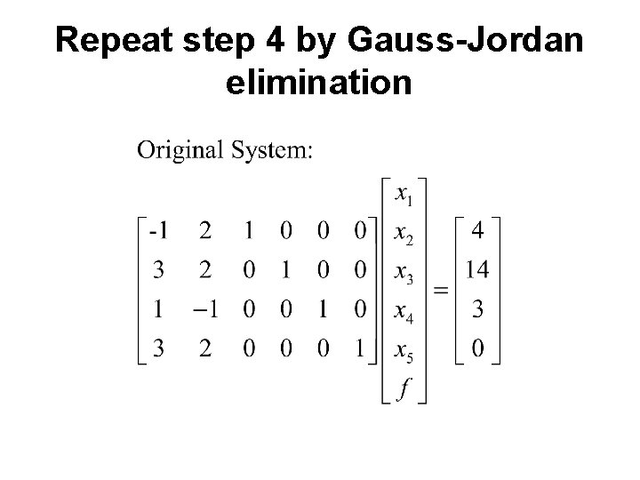
Repeat step 4 by Gauss-Jordan elimination

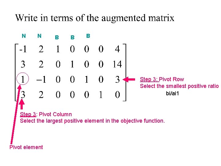
N N B B B Step 3: Pivot Row Select the smallest positive ratio bi/ai 1 Step 3: Pivot Column Select the largest positive element in the objective function. Pivot element

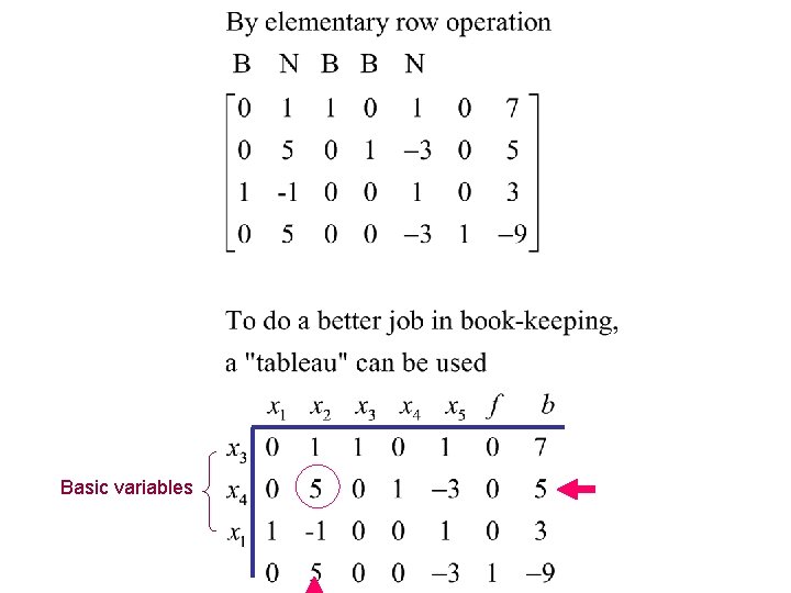
Basic variables

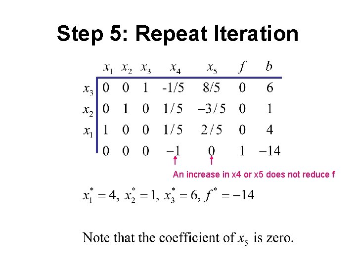
Step 5: Repeat Iteration An increase in x 4 or x 5 does not reduce f

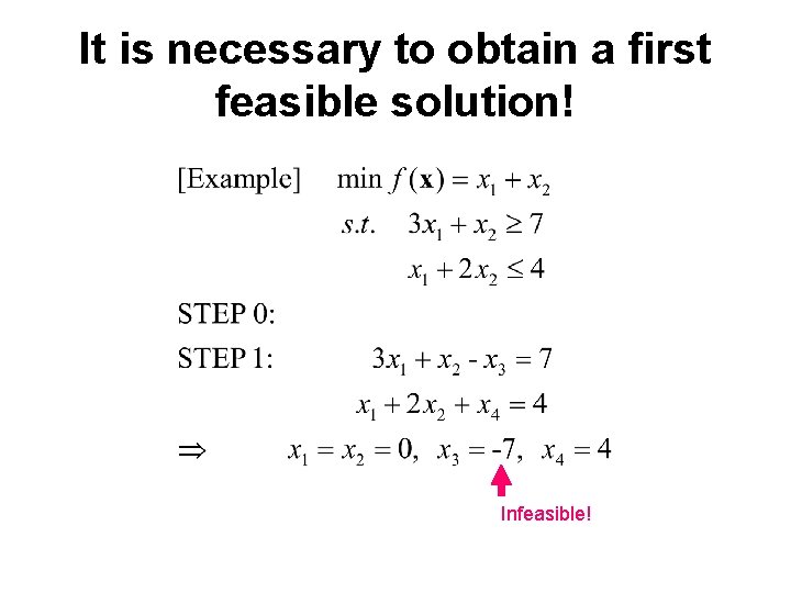
It is necessary to obtain a first feasible solution! Infeasible!

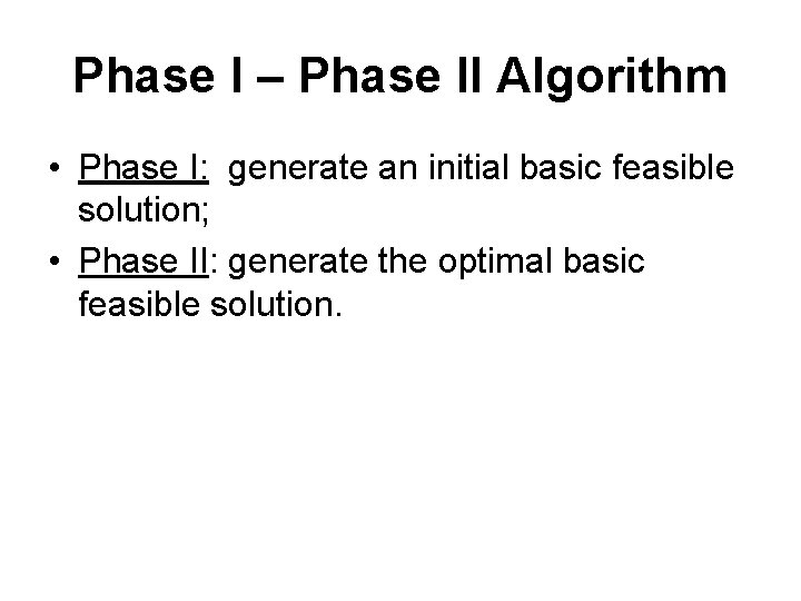
Phase I – Phase II Algorithm • Phase I: generate an initial basic feasible solution; • Phase II: generate the optimal basic feasible solution.

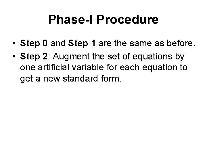
Phase-I Procedure • Step 0 and Step 1 are the same as before. • Step 2: Augment the set of equations by one artificial variable for each equation to get a new standard form.

New Basic Variables

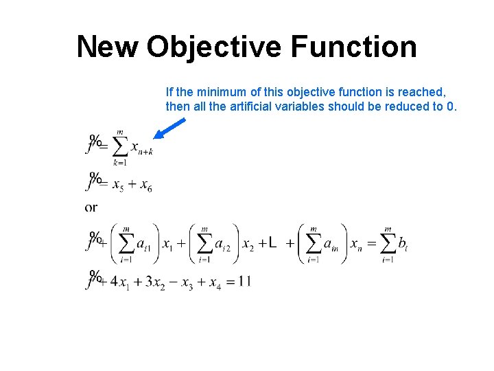
New Objective Function If the minimum of this objective function is reached, then all the artificial variables should be reduced to 0.

Step 3 – Step 5