Part 1 The Prolog Language Chapter 9 Operations

Part 1 The Prolog Language Chapter 9 Operations on Data Structure 1

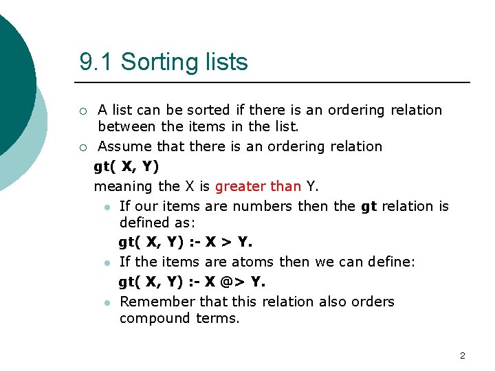
9. 1 Sorting lists ¡ ¡ A list can be sorted if there is an ordering relation between the items in the list. Assume that there is an ordering relation gt( X, Y) meaning the X is greater than Y. l If our items are numbers then the gt relation is defined as: gt( X, Y) : - X > Y. l If the items are atoms then we can define: gt( X, Y) : - X @> Y. l Remember that this relation also orders compound terms. 2

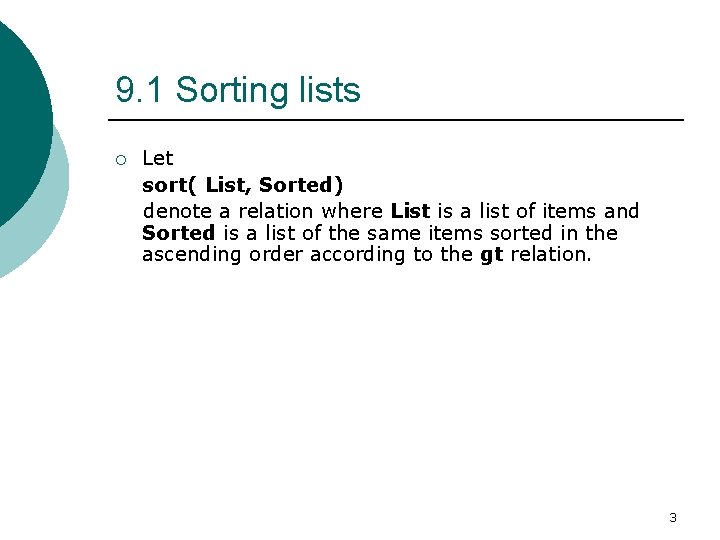
9. 1 Sorting lists ¡ Let sort( List, Sorted) denote a relation where List is a list of items and Sorted is a list of the same items sorted in the ascending order according to the gt relation. 3

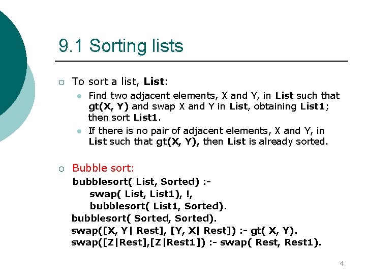
9. 1 Sorting lists ¡ To sort a list, List: l l ¡ Find two adjacent elements, X and Y, in List such that gt(X, Y) and swap X and Y in List, obtaining List 1; then sort List 1. If there is no pair of adjacent elements, X and Y, in List such that gt(X, Y), then List is already sorted. Bubble sort: bubblesort( List, Sorted) : swap( List, List 1), !, bubblesort( List 1, Sorted). bubblesort( Sorted, Sorted). swap([X, Y| Rest], [Y, X| Rest]) : - gt( X, Y). swap([Z|Rest], [Z|Rest 1]) : - swap( Rest, Rest 1). 4

9. 1 Sorting lists | ? - bubblesort([3, 5, 2, 4], L). 1 1 Call: bubblesort([3, 5, 2, 4], _24) ? 2 2 Call: swap([3, 5, 2, 4], _93) ? 3 3 Call: gt(3, 5) ? 4 4 Call: 3>5 ? 4 4 Fail: 3>5 ? 3 3 Fail: gt(3, 5) ? 3 3 Call: swap([5, 2, 4], _80) ? 4 4 Call: gt(5, 2) ? 5 5 Call: 5>2 ? 5 5 Exit: 5>2 ? 4 4 Exit: gt(5, 2) ? 3 3 Exit: swap([5, 2, 4], [2, 5, 4]) ? 2 2 Exit: swap([3, 5, 2, 4], [3, 2, 5, 4]) ? 6 2 Call: bubblesort([3, 2, 5, 4], _24) ? 7 3 Call: swap([3, 2, 5, 4], _223) ? 8 4 Call: gt(3, 2) ? 9 5 Call: 3>2 ? 9 5 Exit: 3>2 ? 8 4 Exit: gt(3, 2) ? 7 3 Exit: swap([3, 2, 5, 4], [2, 3, 5, 4]) ? 10 3 Call: bubblesort([2, 3, 5, 4], _24) ? 11 4 Call: swap([2, 3, 5, 4], _326) ? 12 5 Call: gt(2, 3) ? 13 6 Call: 2>3 ? 13 6 Fail: 2>3 ? 12 5 Fail: gt(2, 3) ? 12 5 Call: swap([3, 5, 4], _313) ? 13 6 Call: gt(3, 5) ? 14 7 Call: 3>5 ? 14 7 Fail: 3>5 ? 13 6 Fail: gt(3, 5) ? 13 6 Call: swap([5, 4], _339) ? 14 7 Call: gt(5, 4) ? 15 8 Call: 5>4 ? 15 8 Exit: 5>4 ? 14 7 Exit: gt(5, 4) ? 13 6 Exit: swap([5, 4], [4, 5]) ? 12 5 Exit: swap([3, 5, 4], [3, 4, 5]) ? 11 4 Exit: swap([2, 3, 5, 4], [2, 3, 4, 5]) ? 16 4 Call: bubblesort([2, 3, 4, 5], _24) ? 17 5 Call: swap([2, 3, 4, 5], _483) ? 18 6 Call: gt(2, 3) ? 19 7 Call: 2>3 ? 19 7 Fail: 2>3 ? 18 6 Fail: gt(2, 3) ? 18 6 Call: swap([3, 4, 5], _470) ? 19 7 Call: gt(3, 4) ? 20 8 Call: 3>4 ? 20 8 Fail: 3>4 ? 19 7 Fail: gt(3, 4) ? 19 7 Call: swap([4, 5], _496) ? 20 8 Call: gt(4, 5) ? 21 9 Call: 4>5 ? 21 9 Fail: 4>5 ? 20 8 Fail: gt(4, 5) ? 20 8 Call: swap([5], _522) ? 21 9 Call: swap([], _548) ? 21 9 Fail: swap([], _548) ? 20 8 Fail: swap([5], _522) ? 19 7 Fail: swap([4, 5], _496) ? 18 6 Fail: swap([3, 4, 5], _470) ? 17 5 Fail: swap([2, 3, 4, 5], _471) ? 16 4 Exit: bubblesort([2, 3, 4, 5], [2, 3, 4, 5]) ? 10 3 Exit: bubblesort([2, 3, 5, 4], [2, 3, 4, 5]) ? 6 2 Exit: bubblesort([3, 2, 5, 4], [2, 3, 4, 5]) ? 1 1 Exit: bubblesort([3, 5, 2, 4], [2, 3, 4, 5]) ? L = [2, 3, 4, 5] (94 ms) yes {trace} 5

9. 1 Sorting lists ¡ To sort a non-empty list, L = [X|T]: l l ¡ Sort the tail T of L. Insert the head, X, of L into the sorted tail at such a position that the resulting list is sorted. The result is the whole sorted list. Insertion sort: insertsort( [], []). insertsort( [X|Tail], Sorted) : insertsort( Tail, Sorted. Tail), insert( X, Sorted. Tail, Sorted). insert(X, [Y| Sorted], [Y| Sorted 1]) : gt( X, Y), !, insert( X, Sorted 1). insert(X, Sorted, [X|Sorted]). 6

9. 1 Sorting lists | ? - insertsort([3, 5, 2, 4], L). 1 1 Call: insertsort([3, 5, 2, 4], _24) ? 2 2 Call: insertsort([5, 2, 4], _93) ? 3 3 Call: insertsort([2, 4], _117) ? 4 4 Call: insertsort([4], _141) ? 5 5 Call: insertsort([], _165) ? 5 5 Exit: insertsort([], []) ? 6 5 Call: insert(4, [], _191) ? 6 5 Exit: insert(4, [], [4]) ? 4 4 Exit: insertsort([4], [4]) ? 7 4 Call: insert(2, [4], _220) ? 8 5 Call: gt(2, 4) ? 9 6 Call: 2>4 ? 9 6 Fail: 2>4 ? 8 5 Fail: gt(2, 4) ? 7 4 Exit: insert(2, [4], [2, 4]) ? 3 3 Exit: insertsort([2, 4], [2, 4]) ? 8 3 Call: insert(5, [2, 4], _249) ? 9 4 Call: gt(5, 2) ? 10 5 Call: 5>2 ? 10 5 Exit: 5>2 ? 9 4 Exit: gt(5, 2) ? 11 4 Call: insert(5, [4], _236) ? 12 5 Call: gt(5, 4) ? 13 6 Call: 5>4 ? 13 6 Exit: 5>4 ? 12 5 Exit: gt(5, 4) ? 14 5 Call: insert(5, [], _313) ? 14 5 Exit: insert(5, [], [5]) ? 11 4 Exit: insert(5, [4], [4, 5]) ? 8 3 Exit: insert(5, [2, 4], [2, 4, 5]) ? 2 2 Exit: insertsort([5, 2, 4], [2, 4, 5]) ? 15 2 Call: insert(3, [2, 4, 5], _24) ? 16 3 Call: gt(3, 2) ? 17 4 Call: 3>2 ? 17 4 Exit: 3>2 ? 16 3 Exit: gt(3, 2) ? 18 3 Call: insert(3, [4, 5], _421) ? 19 4 Call: gt(3, 4) ? 20 5 Call: 3>4 ? 20 5 Fail: 3>4 ? 19 4 Fail: gt(3, 4) ? 18 3 Exit: insert(3, [4, 5], [3, 4, 5]) ? 15 2 Exit: insert(3, [2, 4, 5], [2, 3, 4, 5]) ? 1 1 Exit: insertsort([3, 5, 2, 4], [2, 3, 4, 5]) ? L = [2, 3, 4, 5] (94 ms) yes {trace} 7

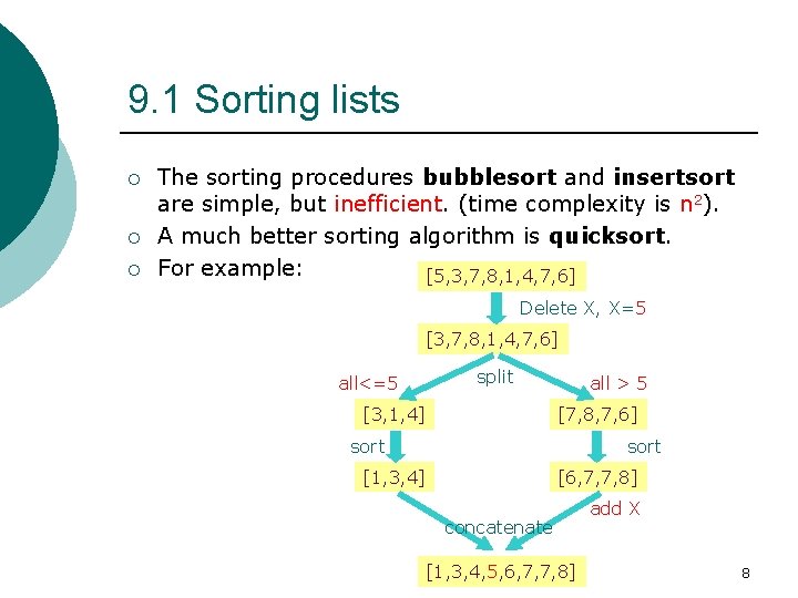
9. 1 Sorting lists ¡ ¡ ¡ The sorting procedures bubblesort and insertsort are simple, but inefficient. (time complexity is n 2). A much better sorting algorithm is quicksort. For example: [5, 3, 7, 8, 1, 4, 7, 6] Delete X, X=5 [3, 7, 8, 1, 4, 7, 6] all<=5 split [3, 1, 4] all > 5 [7, 8, 7, 6] sort [1, 3, 4] [6, 7, 7, 8] concatenate [1, 3, 4, 5, 6, 7, 7, 8] add X 8

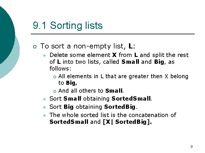
9. 1 Sorting lists ¡ To sort a non-empty list, L: l Delete some element X from L and split the rest of L into two lists, called Small and Big, as follows: ¡ ¡ l l l All elements in L that are greater then X belong to Big, And all others to Small. Sort Small obtaining Sorted. Small. Sort Big obtaining Sorted. Big. The whole sorted list is the concatenation of Sorted. Small and [X| Sorted. Big]. 9

9. 1 Sorting lists ¡ Quick sort: % Figure 9. 2 Quicksort. quicksort( [], []). quicksort( [X|Tail], Sorted) : split( X, Tail, Small, Big), quicksort( Small, Sorted. Small), quicksort( Big, Sorted. Big), conc( Sorted. Small, [X|Sorted. Big], Sorted). split( X, [], []). split( X, [Y|Tail], [Y|Small], Big) : gt( X, Y), !, split( X, Tail, Small, Big). split( X, [Y|Tail], Small, [Y|Big]) : split( X, Tail, Small, Big). 10

9. 1 Sorting lists | ? - quicksort([3, 5, 2, 4], L). 1 1 Call: quicksort([3, 5, 2, 4], _24) ? 2 2 Call: split(3, [5, 2, 4], _95, _96) ? 3 3 Call: gt(3, 5) ? 4 4 Call: 3>5 ? 4 4 Fail: 3>5 ? 3 3 Fail: gt(3, 5) ? 3 3 Call: split(3, [2, 4], _123, _82) ? 4 4 Call: gt(3, 2) ? 5 5 Call: 3>2 ? 5 5 Exit: 3>2 ? 4 4 Exit: gt(3, 2) ? 6 4 Call: split(3, [4], _110, _82) ? 7 5 Call: gt(3, 4) ? 8 6 Call: 3>4 ? 8 6 Fail: 3>4 ? 7 5 Fail: gt(3, 4) ? 7 5 Call: split(3, [], _110, _188) ? 7 5 Exit: split(3, [], []) ? 6 4 Exit: split(3, [4], [4]) ? 3 3 Exit: split(3, [2, 4], [2], [4]) ? 2 2 Exit: split(3, [5, 2, 4], [2], [5, 4]) ? 8 2 Call: quicksort([2], _257) ? 9 3 Call: split(2, [], _283, _284) ? 9 3 Exit: split(2, [], []) ? 10 3 Call: quicksort([], _308) ? 10 3 Exit: quicksort([], []) ? 11 3 Call: quicksort([], _333) ? 11 3 Exit: quicksort([], []) ? 12 3 Call: conc([], [2], _361) ? 12 3 Exit: conc([], [2]) ? 8 2 Exit: quicksort([2], [2]) ? 13 2 Call: quicksort([5, 4], _387) ? 14 3 Call: split(5, [4], _413, _414) ? 15 4 Call: gt(5, 4) ? 16 5 Call: 5>4 ? 16 5 Exit: 5>4 ? 15 4 Exit: gt(5, 4) ? 17 4 Call: split(5, [], _400, _491) ? 17 4 Exit: split(5, [], []) ? 14 3 Exit: split(5, [4], []) ? 18 3 Call: quicksort([4], _517) ? 19 4 Call: split(4, [], _543, _544) ? 19 4 Exit: split(4, [], []) ? 20 4 Call: quicksort([], _568) ? 20 4 Exit: quicksort([], []) ? 21 4 Call: quicksort([], _593) ? 21 4 Exit: quicksort([], []) ? 22 4 Call: conc([], [4], _621) ? 22 4 Exit: conc([], [4]) ? 18 3 Exit: quicksort([4], [4]) ? 23 3 Call: quicksort([], _647) ? 23 3 Exit: quicksort([], []) ? 24 3 Call: conc([4], [5], _675) ? 25 4 Call: conc([], [5], _662) ? 25 4 Exit: conc([], [5]) ? 24 3 Exit: conc([4], [5], [4, 5]) ? 13 2 Exit: quicksort([5, 4], [4, 5]) ? 26 2 Call: conc([2], [3, 4, 5], _24) ? 27 3 Call: conc([], [3, 4, 5], _719) ? 27 3 Exit: conc([], [3, 4, 5]) ? 26 2 Exit: conc([2], [3, 4, 5], [2, 3, 4, 5]) ? 1 1 Exit: quicksort([3, 5, 2, 4], [2, 3, 4, 5]) ? L = [2, 3, 4, 5] ? (78 ms) yes {trace} 11

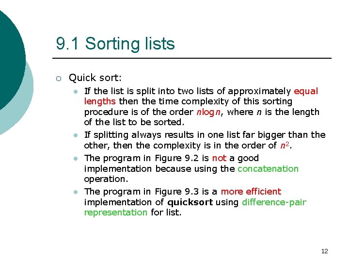
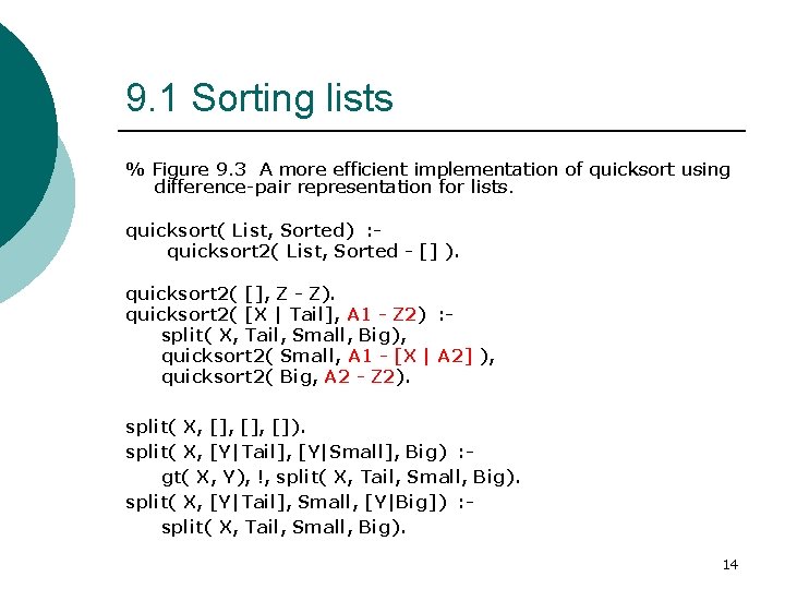
9. 1 Sorting lists ¡ Quick sort: l l If the list is split into two lists of approximately equal lengths then the time complexity of this sorting procedure is of the order nlogn, where n is the length of the list to be sorted. If splitting always results in one list far bigger than the other, then the complexity is in the order of n 2. The program in Figure 9. 2 is not a good implementation because using the concatenation operation. The program in Figure 9. 3 is a more efficient implementation of quicksort using difference-pair representation for list. 12

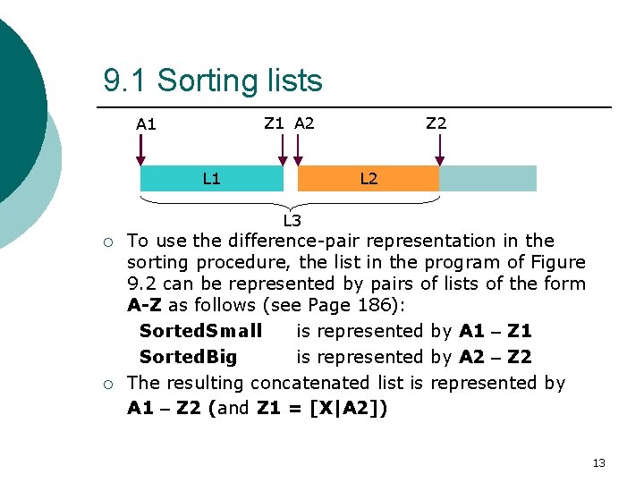
9. 1 Sorting lists Z 1 A 2 A 1 L 1 Z 2 L 3 ¡ ¡ To use the difference-pair representation in the sorting procedure, the list in the program of Figure 9. 2 can be represented by pairs of lists of the form A-Z as follows (see Page 186): Sorted. Small is represented by A 1 – Z 1 Sorted. Big is represented by A 2 – Z 2 The resulting concatenated list is represented by A 1 – Z 2 (and Z 1 = [X|A 2]) 13

9. 1 Sorting lists % Figure 9. 3 A more efficient implementation of quicksort using difference-pair representation for lists. quicksort( List, Sorted) : quicksort 2( List, Sorted - [] ). quicksort 2( [], Z - Z). quicksort 2( [X | Tail], A 1 - Z 2) : split( X, Tail, Small, Big), quicksort 2( Small, A 1 - [X | A 2] ), quicksort 2( Big, A 2 - Z 2). split( X, [], []). split( X, [Y|Tail], [Y|Small], Big) : gt( X, Y), !, split( X, Tail, Small, Big). split( X, [Y|Tail], Small, [Y|Big]) : split( X, Tail, Small, Big). 14

9. 1 Sorting lists |? - quicksort([3, 5, 2, 4], L). 1 2 3 4 5 5 4 4 5 6 6 5 7 8 9 9 8 8 8 7 4 3 9 10 10 11 11 12 1 2 3 4 5 5 4 4 5 6 6 5 5 6 7 7 6 6 6 5 4 3 3 4 4 4 12 4 Exit: quicksort 2([], [3|_250]-[3|_250]) ? 9 3 Exit: quicksort 2([2], [2, 3|_250][3|_250]) ? 13 3 Call: quicksort 2([5, 4], _250 -[]) ? 14 4 Call: split(5, [4], _428, _429) ? 15 5 Call: gt(5, 4) ? 16 6 Call: 5>4 ? 16 6 Exit: 5>4 ? 15 5 Exit: gt(5, 4) ? 17 5 Call: split(5, [], _415, _506) ? 17 5 Exit: split(5, [], []) ? 14 4 Exit: split(5, [4], []) ? 18 4 Call: quicksort 2([4], _250 -[5|_498]) ? 19 5 Call: split(4, [], _563, _564) ? 19 5 Exit: split(4, [], []) ? 20 5 Call: quicksort 2([], _250 -[4|_554]) ? 20 5 Exit: quicksort 2([], [4|_554]-[4|_554]) ? 21 5 Call: quicksort 2([], _554 -[5|_498]) ? 21 5 Exit: quicksort 2([], [5|_498]-[5|_498]) ? 18 4 Exit: quicksort 2([4], [4, 5|_498][5|_498]) ? 22 4 Call: quicksort 2([], _498 -[]) ? 22 4 Exit: quicksort 2([], []-[]) ? 13 3 Exit: quicksort 2([5, 4], [4, 5]-[]) ? 2 2 Exit: quicksort 2([3, 5, 2, 4], [2, 3, 4, 5]-[]) ? 1 1 Exit: quicksort([3, 5, 2, 4], [2, 3, 4, 5]) ? Call: quicksort([3, 5, 2, 4], _24) ? Call: quicksort 2([3, 5, 2, 4], _24 -[]) ? Call: split(3, [5, 2, 4], _122, _123) ? Call: gt(3, 5) ? Call: 3>5 ? Fail: gt(3, 5) ? Call: split(3, [2, 4], _150, _109) ? Call: gt(3, 2) ? Call: 3>2 ? Exit: gt(3, 2) ? Call: split(3, [4], _137, _109) ? Call: gt(3, 4) ? Call: 3>4 ? Fail: gt(3, 4) ? Call: split(3, [], _137, _215) ? Exit: split(3, [], []) ? Exit: split(3, [4], [4]) ? Exit: split(3, [2, 4], [2], [4]) ? Exit: split(3, [5, 2, 4], [2], [5, 4]) ? Call: quicksort 2([2], _24 -[3|_250]) ? Call: split(2, [], _315, _316) ? Exit: split(2, [], []) ? L = [2, 3, 4, 5] ? Call: quicksort 2([], _24 -[2|_306]) ? Exit: quicksort 2([], [2|_306]-[2|_306]) ? (31 ms) yes Call: quicksort 2([], _306 -[3|_250]) ? {trace} 15

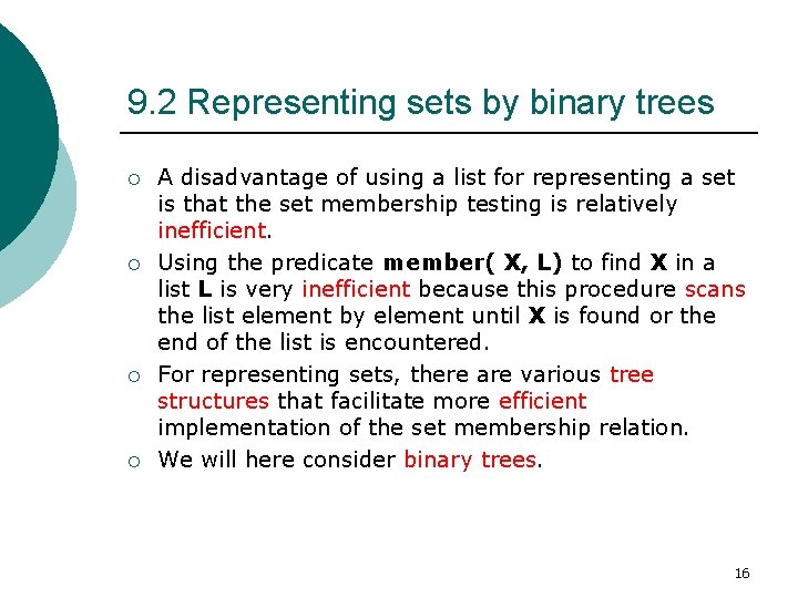
9. 2 Representing sets by binary trees ¡ ¡ A disadvantage of using a list for representing a set is that the set membership testing is relatively inefficient. Using the predicate member( X, L) to find X in a list L is very inefficient because this procedure scans the list element by element until X is found or the end of the list is encountered. For representing sets, there are various tree structures that facilitate more efficient implementation of the set membership relation. We will here consider binary trees. 16

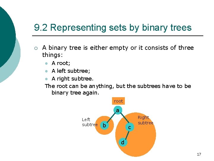
9. 2 Representing sets by binary trees ¡ A binary tree is either empty or it consists of three things: A root; l A left subtree; l A right subtree. The root can be anything, but the subtrees have to be binary tree again. l root a Left subtree b c Right subtree d 17

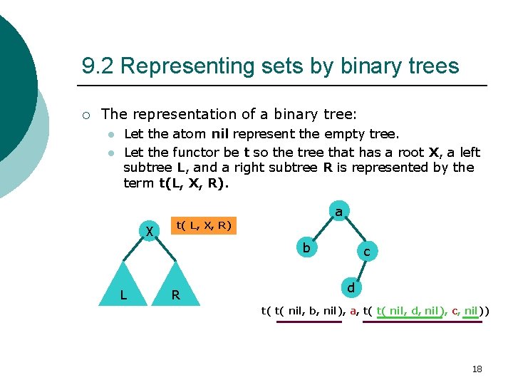
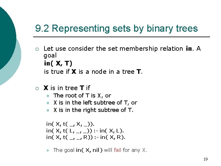
9. 2 Representing sets by binary trees ¡ The representation of a binary tree: l l Let the atom nil represent the empty tree. Let the functor be t so the tree that has a root X, a left subtree L, and a right subtree R is represented by the term t(L, X, R). a X t( L, X, R) b L R c d t( t( nil, b, nil), a, t( t( nil, d, nil), c, nil)) 18

9. 2 Representing sets by binary trees ¡ Let use consider the set membership relation in. A goal in( X, T) is true if X is a node in a tree T. ¡ X is in tree T if l l l The root of T is X, or X is in the left subtree of T, or X is in the right subtree of T. in( X, t( _, X, _)). in( X, t( L, _, _)) : - in( X, L). in( X, t( _, _, R)) : - in( X, R). l The goal in( X, nil) will fail for any X. 19

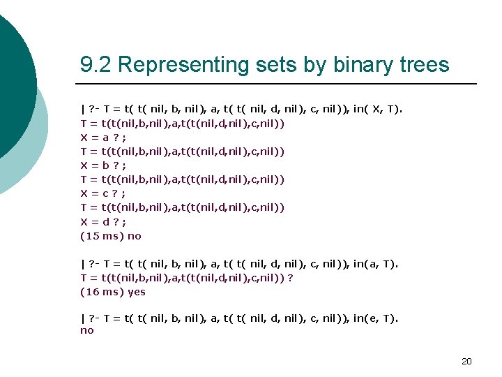
9. 2 Representing sets by binary trees | ? - T = t( t( nil, b, nil), a, t( t( nil, d, nil), c, nil)), in( X, T). T = t(t(nil, b, nil), a, t(t(nil, d, nil), c, nil)) X=a? ; T = t(t(nil, b, nil), a, t(t(nil, d, nil), c, nil)) X=b? ; T = t(t(nil, b, nil), a, t(t(nil, d, nil), c, nil)) X=c? ; T = t(t(nil, b, nil), a, t(t(nil, d, nil), c, nil)) X=d? ; (15 ms) no | ? - T = t( t( nil, b, nil), a, t( t( nil, d, nil), c, nil)), in(a, T). T = t(t(nil, b, nil), a, t(t(nil, d, nil), c, nil)) ? (16 ms) yes | ? - T = t( t( nil, b, nil), a, t( t( nil, d, nil), c, nil)), in(e, T). no 20

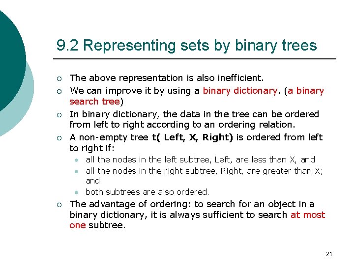
9. 2 Representing sets by binary trees ¡ ¡ The above representation is also inefficient. We can improve it by using a binary dictionary. (a binary search tree) In binary dictionary, the data in the tree can be ordered from left to right according to an ordering relation. A non-empty tree t( Left, X, Right) is ordered from left to right if: l l l ¡ all the nodes in the left subtree, Left, are less than X, and all the nodes in the right subtree, Right, are greater than X; and both subtrees are also ordered. The advantage of ordering: to search for an object in a binary dictionary, it is always sufficient to search at most one subtree. 21

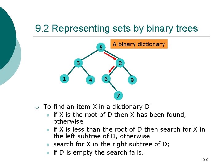
9. 2 Representing sets by binary trees A binary dictionary 5 3 1 8 4 6 9 7 ¡ To find an item X in a dictionary D: l if X is the root of D then X has been found, otherwise l if X is less than the root of D then search for X in the left subtree of D, otherwise l search for X in the right subtree of D; l if D is empty the search fails. 22

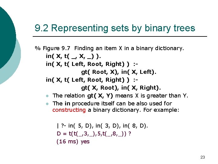
9. 2 Representing sets by binary trees % Figure 9. 7 Finding an item X in a binary dictionary. in( X, t( _, X, _) ). in( X, t( Left, Root, Right) ) : gt( Root, X), in( X, Left). in( X, t( Left, Root, Right) ) : gt( X, Root), in( X, Right). l The relation gt( X, Y) means X is greater than Y. l The in procedure itself can be also used for constructing a binary dictionary. For example: | ? - in( 5, D), in( 3, D), in( 8, D). D = t(t(_, 3, _), 5, t(_, 8, _)) ? (16 ms) yes 23

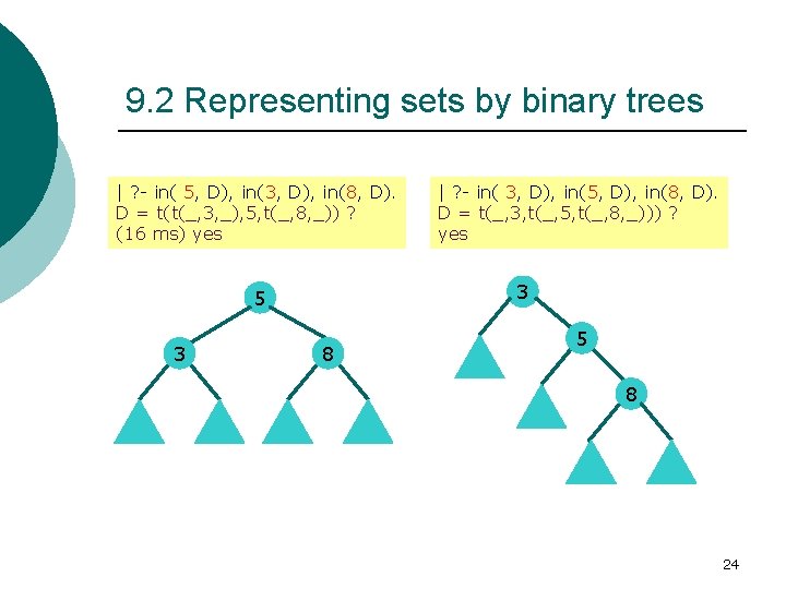
9. 2 Representing sets by binary trees | ? - in( 5, D), in(3, D), in(8, D). D = t(t(_, 3, _), 5, t(_, 8, _)) ? (16 ms) yes 3 5 3 | ? - in( 3, D), in(5, D), in(8, D). D = t(_, 3, t(_, 5, t(_, 8, _))) ? yes 8 5 8 24

9. 2 Representing sets by binary trees ¡ ¡ A tree is (approximately) balanced if, for each node in the tree, its two subtrees accommodate(容納) an approximately equal number of items. If a dictionary with n nodes is nicely balanced then its height is proportional to logn. If the tree gets out of balance its performance will degrade. In extreme cases of totally unbalanced trees, a tree is reduced to a list. In such a case the tree’s height is n, and the tree’s performance is equally poor as that of a list. 25

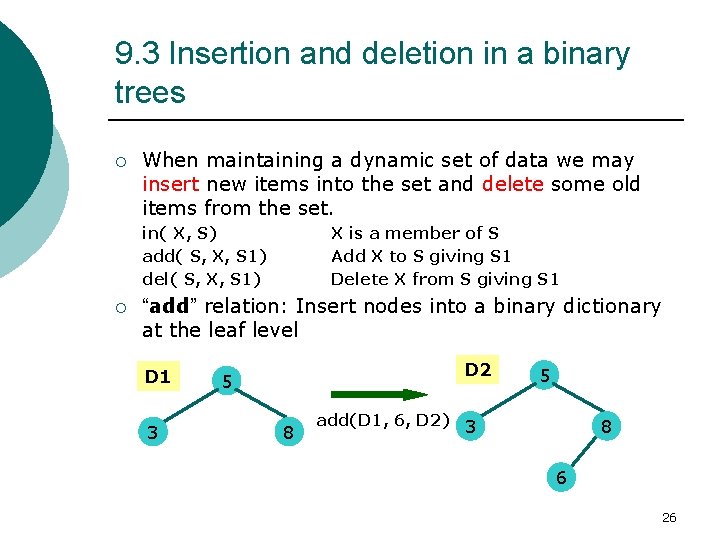
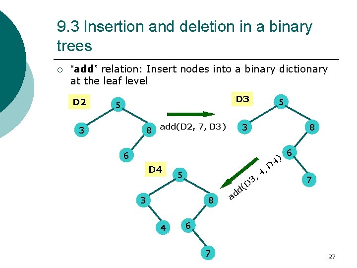
9. 3 Insertion and deletion in a binary trees ¡ When maintaining a dynamic set of data we may insert new items into the set and delete some old items from the set. in( X, S) add( S, X, S 1) del( S, X, S 1) ¡ X is a member of S Add X to S giving S 1 Delete X from S giving S 1 “add” relation: Insert nodes into a binary dictionary at the leaf level D 1 3 D 2 5 8 5 add(D 1, 6, D 2) 3 8 6 26

9. 3 Insertion and deletion in a binary trees ¡ “add” relation: Insert nodes into a binary dictionary at the leaf level D 2 D 3 5 8 add(D 2, 7, D 3) 3 5 3 8 6 D 4 5 3 3 8 4 , , 4 (D d ad D 4) 6 7 27

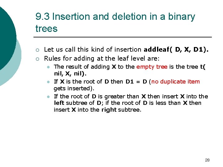
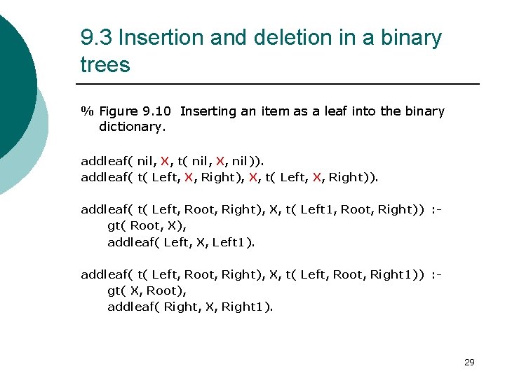
9. 3 Insertion and deletion in a binary trees ¡ ¡ Let us call this kind of insertion addleaf( D, X, D 1). Rules for adding at the leaf level are: l l l The result of adding X to the empty tree is the tree t( nil, X, nil). If X is the root of D then D 1 = D (no duplicate item gets inserted). If the root of D is greater than X then insert X into the left subtree of D; if the root of D is less than X then insert X into the right subtree. 28

9. 3 Insertion and deletion in a binary trees % Figure 9. 10 Inserting an item as a leaf into the binary dictionary. addleaf( nil, X, t( nil, X, nil)). addleaf( t( Left, X, Right), X, t( Left, X, Right)). addleaf( t( Left, Root, Right), X, t( Left 1, Root, Right)) : gt( Root, X), addleaf( Left, X, Left 1). addleaf( t( Left, Root, Right), X, t( Left, Root, Right 1)) : gt( X, Root), addleaf( Right, X, Right 1). 29

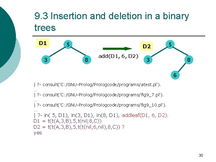
9. 3 Insertion and deletion in a binary trees D 1 3 5 D 2 8 add(D 1, 6, D 2) 5 3 8 6 | ? - consult('C: /GNU-Prolog/Prologcode/programs/atest. pl'). … | ? - consult('C: /GNU-Prolog/Prologcode/programs/fig 9_7. pl'). … | ? - consult('C: /GNU-Prolog/Prologcode/programs/fig 9_10. pl'). … | ? - in( 5, D 1), in(3, D 1), in(8, D 1), addleaf(D 1, 6, D 2). D 1 = t(t(A, 3, B), 5, t(nil, 8, C)) D 2 = t(t(A, 3, B), 5, t(t(nil, 6, nil), 8, C)) ? yes 30

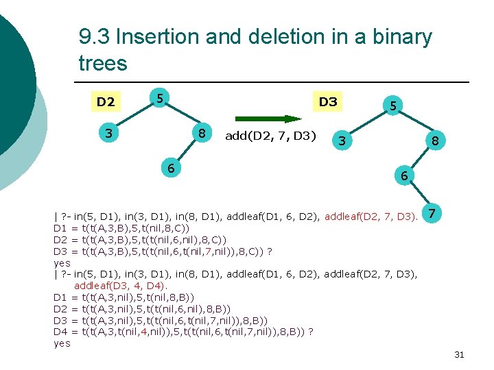
9. 3 Insertion and deletion in a binary trees D 2 5 D 3 3 8 6 add(D 2, 7, D 3) 5 3 8 6 | ? - in(5, D 1), in(3, D 1), in(8, D 1), addleaf(D 1, 6, D 2), addleaf(D 2, 7, D 3). D 1 = t(t(A, 3, B), 5, t(nil, 8, C)) D 2 = t(t(A, 3, B), 5, t(t(nil, 6, nil), 8, C)) D 3 = t(t(A, 3, B), 5, t(t(nil, 6, t(nil, 7, nil)), 8, C)) ? yes | ? - in(5, D 1), in(3, D 1), in(8, D 1), addleaf(D 1, 6, D 2), addleaf(D 2, 7, D 3), addleaf(D 3, 4, D 4). D 1 = t(t(A, 3, nil), 5, t(nil, 8, B)) D 2 = t(t(A, 3, nil), 5, t(t(nil, 6, nil), 8, B)) D 3 = t(t(A, 3, nil), 5, t(t(nil, 6, t(nil, 7, nil)), 8, B)) D 4 = t(t(A, 3, t(nil, 4, nil)), 5, t(t(nil, 6, t(nil, 7, nil)), 8, B)) ? yes 7 31

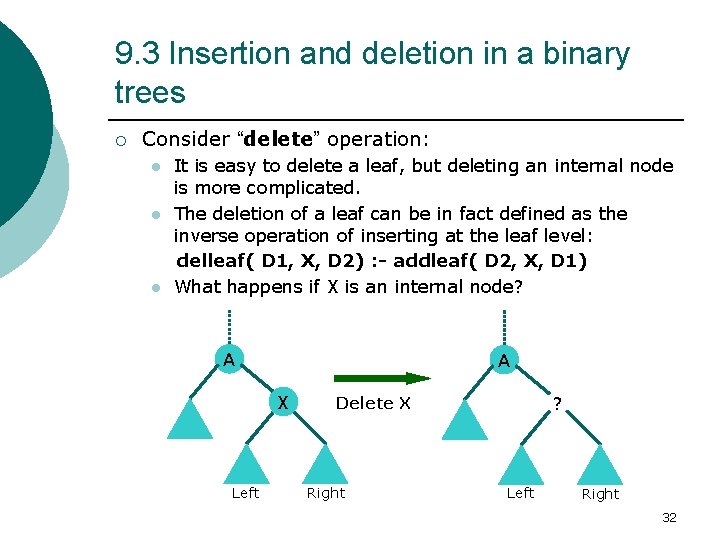
9. 3 Insertion and deletion in a binary trees ¡ Consider “delete” operation: l l l It is easy to delete a leaf, but deleting an internal node is more complicated. The deletion of a leaf can be in fact defined as the inverse operation of inserting at the leaf level: delleaf( D 1, X, D 2) : - addleaf( D 2, X, D 1) What happens if X is an internal node? A A X Left ? Delete X Right Left Right 32

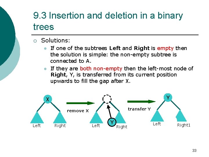
9. 3 Insertion and deletion in a binary trees ¡ Solutions: l l If one of the subtrees Left and Right is empty then the solution is simple: the non-empty subtree is connected to A. If they are both non-empty then the left-most node of Right, Y, is transferred from its current position upwards to fill the gap after X. Y X transfer Y remove X Left Right Left Y Right Left Right 1 33

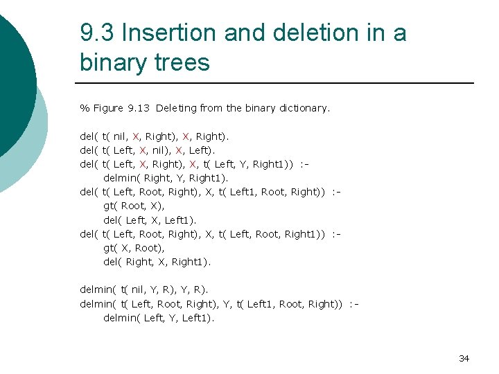
9. 3 Insertion and deletion in a binary trees % Figure 9. 13 Deleting from the binary dictionary. del( t( nil, X, Right). del( t( Left, X, nil), X, Left). del( t( Left, X, Right), X, t( Left, Y, Right 1)) : delmin( Right, Y, Right 1). del( t( Left, Root, Right), X, t( Left 1, Root, Right)) : gt( Root, X), del( Left, X, Left 1). del( t( Left, Root, Right), X, t( Left, Root, Right 1)) : gt( X, Root), del( Right, X, Right 1). delmin( t( nil, Y, R). delmin( t( Left, Root, Right), Y, t( Left 1, Root, Right)) : delmin( Left, Y, Left 1). 34

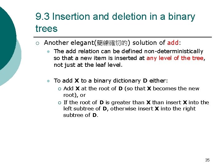
9. 3 Insertion and deletion in a binary trees ¡ Another elegant(簡練確切的) solution of add: l The add relation can be defined non-deterministically so that a new item is inserted at any level of the tree, not just at the leaf level. l To add X to a binary dictionary D either: ¡ ¡ Add X at the root of D (so that X becomes the new root), or If the root of D is greater than X than insert X into the left subtree of D, otherwise insert X into the right subtree of D. 35

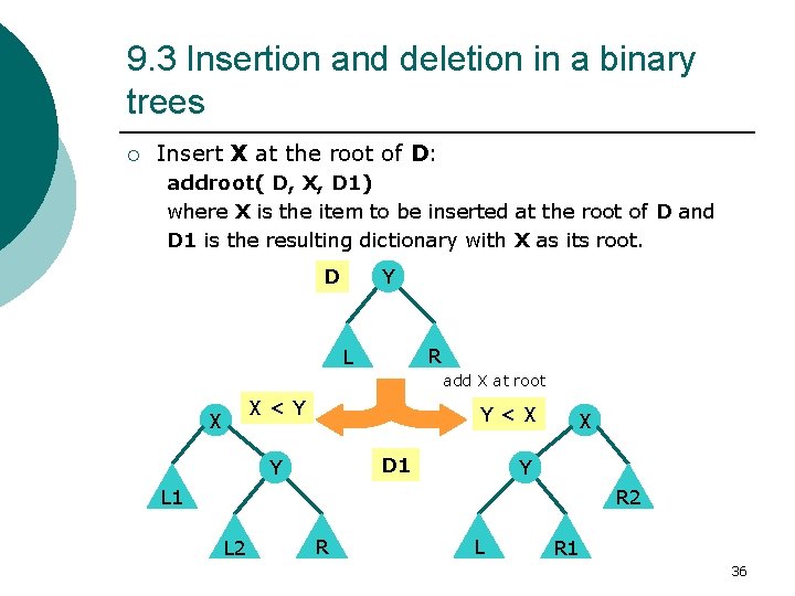
9. 3 Insertion and deletion in a binary trees ¡ Insert X at the root of D: addroot( D, X, D 1) where X is the item to be inserted at the root of D and D 1 is the resulting dictionary with X as its root. Y D R L add X at root X<Y X Y<X D 1 Y X Y L 1 R 2 L 2 R L R 1 36

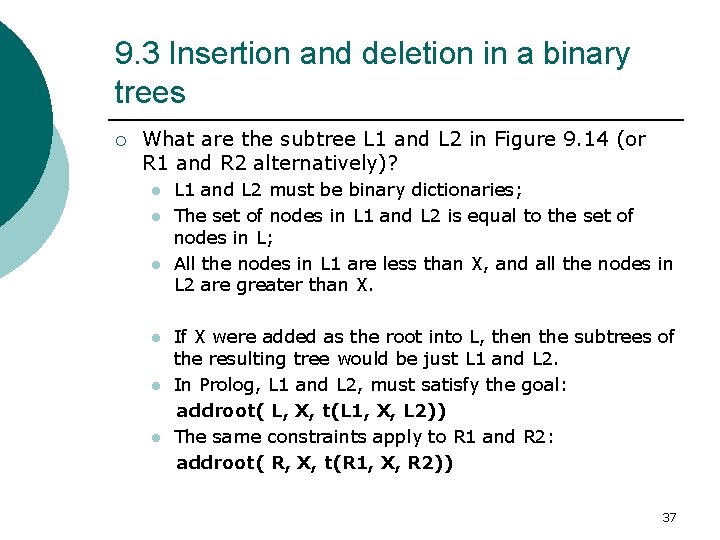
9. 3 Insertion and deletion in a binary trees ¡ What are the subtree L 1 and L 2 in Figure 9. 14 (or R 1 and R 2 alternatively)? l l l L 1 and L 2 must be binary dictionaries; The set of nodes in L 1 and L 2 is equal to the set of nodes in L; All the nodes in L 1 are less than X, and all the nodes in L 2 are greater than X. If X were added as the root into L, then the subtrees of the resulting tree would be just L 1 and L 2. In Prolog, L 1 and L 2, must satisfy the goal: addroot( L, X, t(L 1, X, L 2)) The same constraints apply to R 1 and R 2: addroot( R, X, t(R 1, X, R 2)) 37

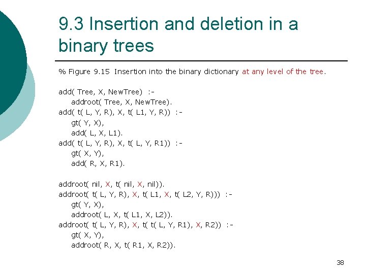
9. 3 Insertion and deletion in a binary trees % Figure 9. 15 Insertion into the binary dictionary at any level of the tree. add( Tree, X, New. Tree) : addroot( Tree, X, New. Tree). add( t( L, Y, R), X, t( L 1, Y, R)) : gt( Y, X), add( L, X, L 1). add( t( L, Y, R), X, t( L, Y, R 1)) : gt( X, Y), add( R, X, R 1). addroot( nil, X, nil)). addroot( t( L, Y, R), X, t( L 1, X, t( L 2, Y, R))) : gt( Y, X), addroot( L, X, t( L 1, X, L 2)). addroot( t( L, Y, R), X, t( t( L, Y, R 1), X, R 2)) : gt( X, Y), addroot( R, X, t( R 1, X, R 2)). 38

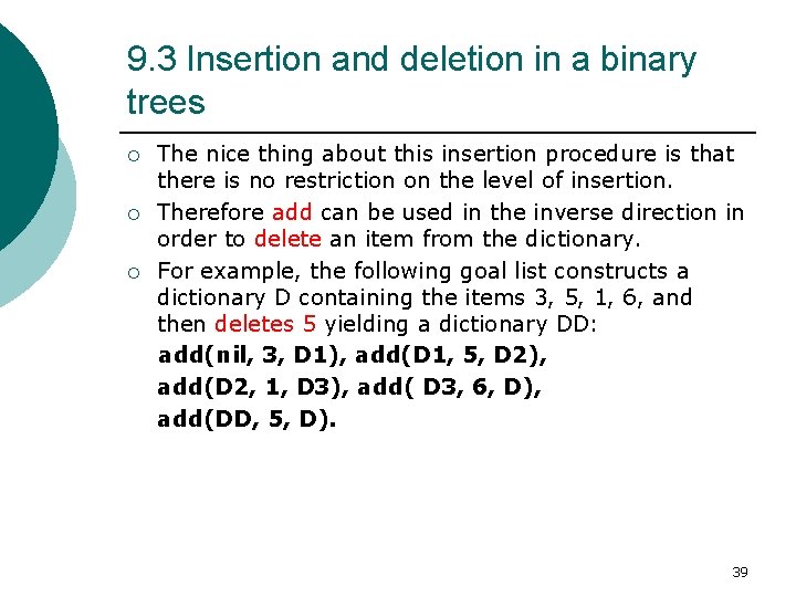
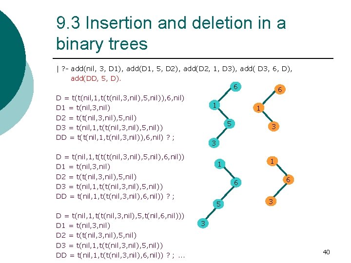
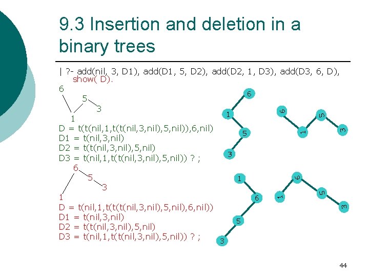
9. 3 Insertion and deletion in a binary trees ¡ ¡ ¡ The nice thing about this insertion procedure is that there is no restriction on the level of insertion. Therefore add can be used in the inverse direction in order to delete an item from the dictionary. For example, the following goal list constructs a dictionary D containing the items 3, 5, 1, 6, and then deletes 5 yielding a dictionary DD: add(nil, 3, D 1), add(D 1, 5, D 2), add(D 2, 1, D 3), add( D 3, 6, D), add(DD, 5, D). 39

9. 3 Insertion and deletion in a binary trees | ? - add(nil, 3, D 1), add(D 1, 5, D 2), add(D 2, 1, D 3), add( D 3, 6, D), add(DD, 5, D). 6 6 D = t(t(nil, 1, t(t(nil, 3, nil), 5, nil)), 6, nil) 1 D 1 = t(nil, 3, nil) 1 D 2 = t(t(nil, 3, nil), 5, nil) 5 3 D 3 = t(nil, 1, t(t(nil, 3, nil), 5, nil)) DD = t(t(nil, 1, t(nil, 3, nil)), 6, nil) ? ; 3 D = t(nil, 1, t(t(t(nil, 3, nil), 5, nil), 6, nil)) D 1 = t(nil, 3, nil) D 2 = t(t(nil, 3, nil), 5, nil) D 3 = t(nil, 1, t(t(nil, 3, nil), 5, nil)) DD = t(nil, 1, t(t(nil, 3, nil), 6, nil)) ? ; D = t(nil, 1, t(t(nil, 3, nil), 5, t(nil, 6, nil))) D 1 = t(nil, 3, nil) D 2 = t(t(nil, 3, nil), 5, nil) D 3 = t(nil, 1, t(t(nil, 3, nil), 5, nil)) DD = t(nil, 1, t(t(nil, 3, nil), 6, nil)) ? ; . . . 1 1 6 6 5 3 3 40

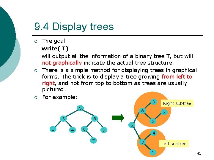
9. 4 Display trees ¡ ¡ ¡ The goal write( T) will output all the information of a binary tree T, but will not graphically indicate the actual tree structure. There is a simple method for displaying trees in graphical forms. The trick is to display a tree growing from left to right, and not from top to bottom as trees are usually pictured. For example: 9 5 8 3 1 8 4 6 9 7 Right subtree 7 6 5 4 3 Left subtree 1 41

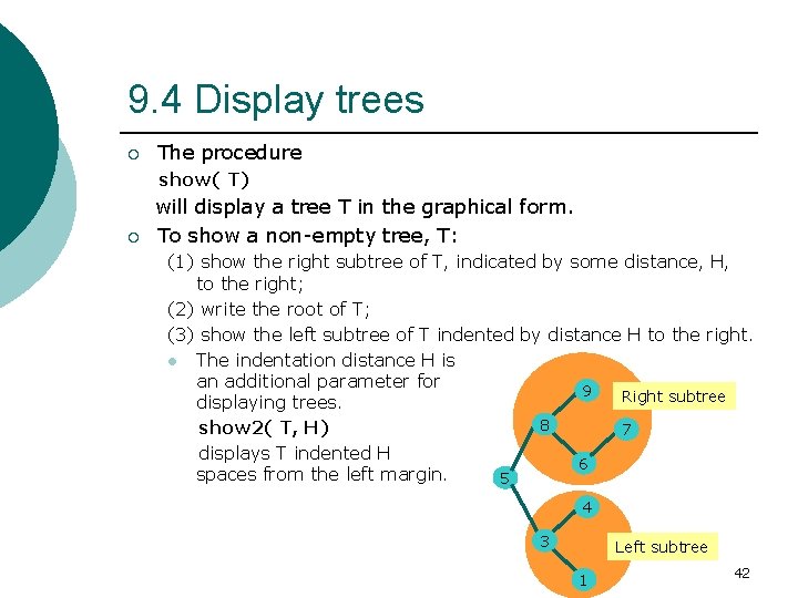
9. 4 Display trees ¡ The procedure show( T) ¡ will display a tree T in the graphical form. To show a non-empty tree, T: (1) show the right subtree of T, indicated by some distance, H, to the right; (2) write the root of T; (3) show the left subtree of T indented by distance H to the right. l The indentation distance H is an additional parameter for 9 Right subtree displaying trees. 8 show 2( T, H) 7 displays T indented H 6 spaces from the left margin. 5 4 3 Left subtree 1 42

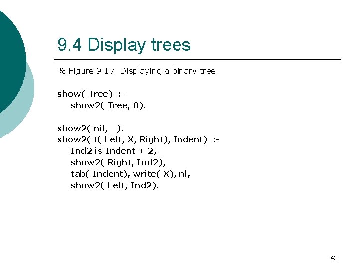
9. 4 Display trees % Figure 9. 17 Displaying a binary tree. show( Tree) : show 2( Tree, 0). show 2( nil, _). show 2( t( Left, X, Right), Indent) : Ind 2 is Indent + 2, show 2( Right, Ind 2), tab( Indent), write( X), nl, show 2( Left, Ind 2). 43

9. 3 Insertion and deletion in a binary trees 3 5 1 6 1 3 5 6 | ? - add(nil, 3, D 1), add(D 1, 5, D 2), add(D 2, 1, D 3), add(D 3, 6, D), show( D). 6 6 5 3 1 1 D = t(t(nil, 1, t(t(nil, 3, nil), 5, nil)), 6, nil) 5 D 1 = t(nil, 3, nil) D 2 = t(t(nil, 3, nil), 5, nil) 3 D 3 = t(nil, 1, t(t(nil, 3, nil), 5, nil)) ? ; 6 5 1 3 1 6 D = t(nil, 1, t(t(t(nil, 3, nil), 5, nil), 6, nil)) D 1 = t(nil, 3, nil) 5 D 2 = t(t(nil, 3, nil), 5, nil) D 3 = t(nil, 1, t(t(nil, 3, nil), 5, nil)) ? ; 3 44

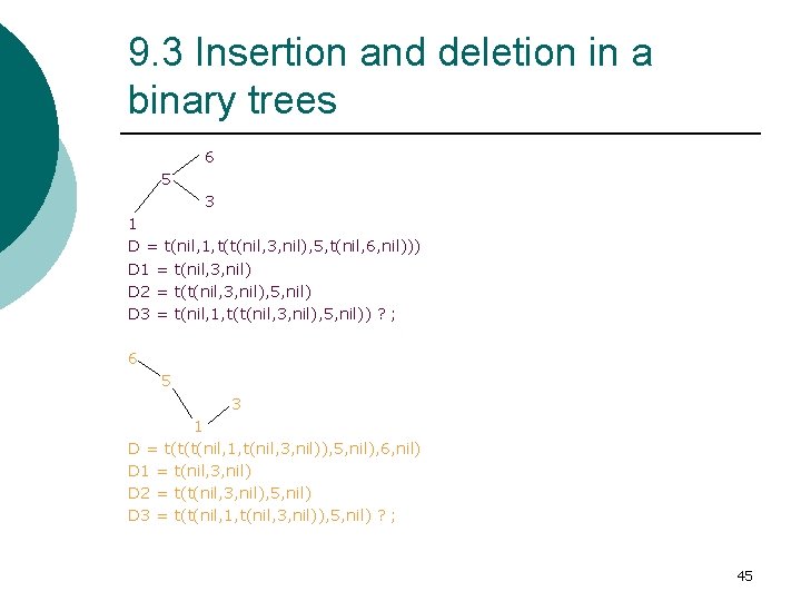
9. 3 Insertion and deletion in a binary trees 6 5 3 1 D = t(nil, 1, t(t(nil, 3, nil), 5, t(nil, 6, nil))) D 1 = t(nil, 3, nil) D 2 = t(t(nil, 3, nil), 5, nil) D 3 = t(nil, 1, t(t(nil, 3, nil), 5, nil)) ? ; 6 5 3 1 D = t(t(t(nil, 1, t(nil, 3, nil)), 5, nil), 6, nil) D 1 = t(nil, 3, nil) D 2 = t(t(nil, 3, nil), 5, nil) D 3 = t(t(nil, 1, t(nil, 3, nil)), 5, nil) ? ; 45

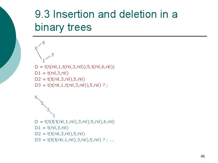
9. 3 Insertion and deletion in a binary trees 6 5 3 1 D = t(t(nil, 1, t(nil, 3, nil)), 5, t(nil, 6, nil)) D 1 = t(nil, 3, nil) D 2 = t(t(nil, 3, nil), 5, nil) D 3 = t(t(nil, 1, t(nil, 3, nil)), 5, nil) ? ; 6 5 3 1 D = t(t(nil, 1, nil), 3, nil), 5, nil), 6, nil) D 1 = t(nil, 3, nil) D 2 = t(t(nil, 3, nil), 5, nil) D 3 = t(t(t(nil, 1, nil), 3, nil), 5, nil) ? ; . . . 46

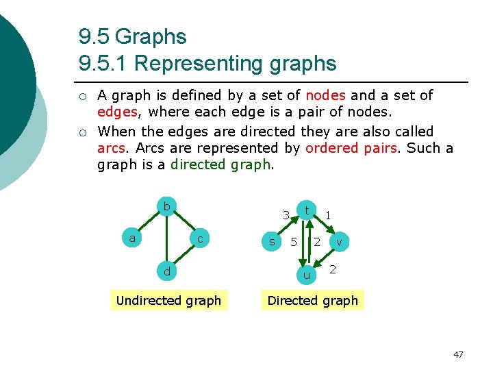
9. 5 Graphs 9. 5. 1 Representing graphs ¡ ¡ A graph is defined by a set of nodes and a set of edges, where each edge is a pair of nodes. When the edges are directed they are also called arcs. Arcs are represented by ordered pairs. Such a graph is a directed graph. b a t 3 c d Undirected graph s 5 1 v 2 u 2 Directed graph 47

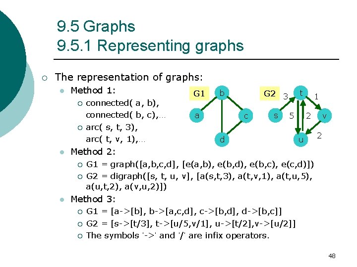
9. 5 Graphs 9. 5. 1 Representing graphs ¡ The representation of graphs: l Method 1: ¡ ¡ l b a t G 2 3 c s 5 d 1 v 2 u 2 Method 2: ¡ ¡ l connected( a, b), connected( b, c), … arc( s, t, 3), arc( t, v, 1), … G 1 = graph([a, b, c, d], [e(a, b), e(b, d), e(b, c), e(c, d)]) G 2 = digraph([s, t, u, v], [a(s, t, 3), a(t, v, 1), a(t, u, 5), a(u, t, 2), a(v, u, 2)]) Method 3: ¡ ¡ ¡ G 1 = [a->[b], b->[a, c, d], c->[b, d], d->[b, c]] G 2 = [s->[t/3], t->[u/5, v/1], u->[t/2], v->[u/2]] The symbols ’->’ and ’/’ are infix operators. 48

9. 5 Graphs 9. 5. 1 Representing graphs ¡ What is the most suitable representation? l ¡ Depending on the application and on operations to be performed on graphs. Two typical operations are: l l Find a path between two given nodes; Find a subgraph, with some specified properties, of a graph. 49

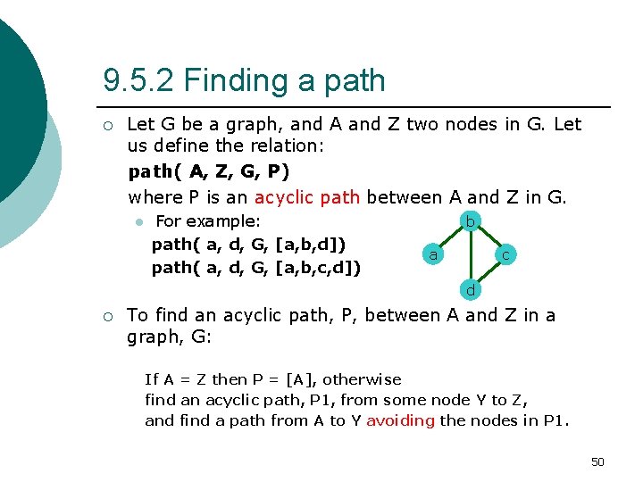
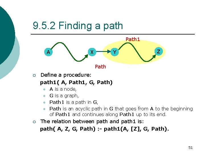
9. 5. 2 Finding a path ¡ Let G be a graph, and A and Z two nodes in G. Let us define the relation: path( A, Z, G, P) where P is an acyclic path between A and Z in G. l For example: path( a, d, G, [a, b, d]) path( a, d, G, [a, b, c, d]) b a c d ¡ To find an acyclic path, P, between A and Z in a graph, G: If A = Z then P = [A], otherwise find an acyclic path, P 1, from some node Y to Z, and find a path from A to Y avoiding the nodes in P 1. 50

9. 5. 2 Finding a path Path 1 A X Y Z Path ¡ Define a procedure: path 1( A, Path 1, G, Path) l l ¡ A is a node, G is a graph, Path 1 is a path in G, Path is an acyclic path in G that goes from A to the beginning of Path 1 and continues along Path 1 up to its end. The relation between path and path 1 is: path( A, Z, G, Path) : - path 1(A, [Z], G, Path). 51

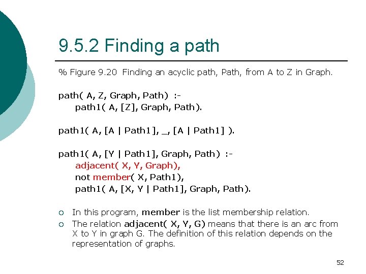
9. 5. 2 Finding a path % Figure 9. 20 Finding an acyclic path, Path, from A to Z in Graph. path( A, Z, Graph, Path) : path 1( A, [Z], Graph, Path). path 1( A, [A | Path 1], _, [A | Path 1] ). path 1( A, [Y | Path 1], Graph, Path) : adjacent( X, Y, Graph), not member( X, Path 1), path 1( A, [X, Y | Path 1], Graph, Path). ¡ ¡ In this program, member is the list membership relation. The relation adjacent( X, Y, G) means that there is an arc from X to Y in graph G. The definition of this relation depends on the representation of graphs. 52

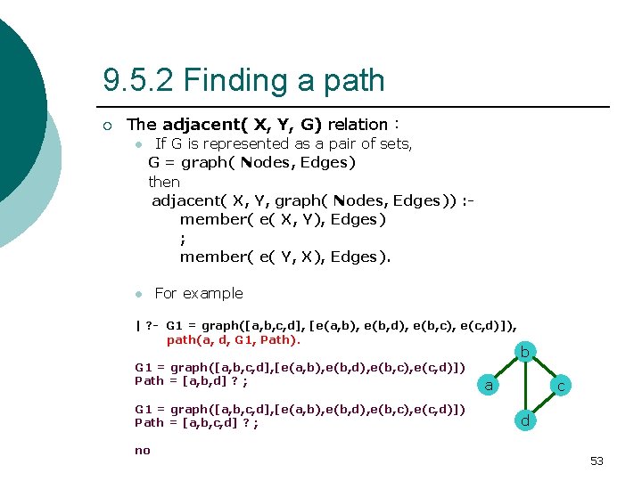
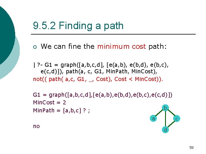
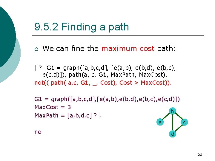
9. 5. 2 Finding a path ¡ The adjacent( X, Y, G) relation： l If G is represented as a pair of sets, G = graph( Nodes, Edges) then adjacent( X, Y, graph( Nodes, Edges)) : member( e( X, Y), Edges) ; member( e( Y, X), Edges). l For example | ? - G 1 = graph([a, b, c, d], [e(a, b), e(b, d), e(b, c), e(c, d)]), path(a, d, G 1, Path). G 1 = graph([a, b, c, d], [e(a, b), e(b, d), e(b, c), e(c, d)]) Path = [a, b, d] ? ; G 1 = graph([a, b, c, d], [e(a, b), e(b, d), e(b, c), e(c, d)]) Path = [a, b, c, d] ? ; no b a c d 53

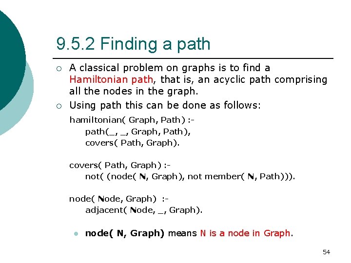
9. 5. 2 Finding a path ¡ ¡ A classical problem on graphs is to find a Hamiltonian path, that is, an acyclic path comprising all the nodes in the graph. Using path this can be done as follows: hamiltonian( Graph, Path) : path(_, _, Graph, Path), covers( Path, Graph) : not( (node( N, Graph), not member( N, Path))). node( Node, Graph) : adjacent( Node, _, Graph). l node( N, Graph) means N is a node in Graph. 54

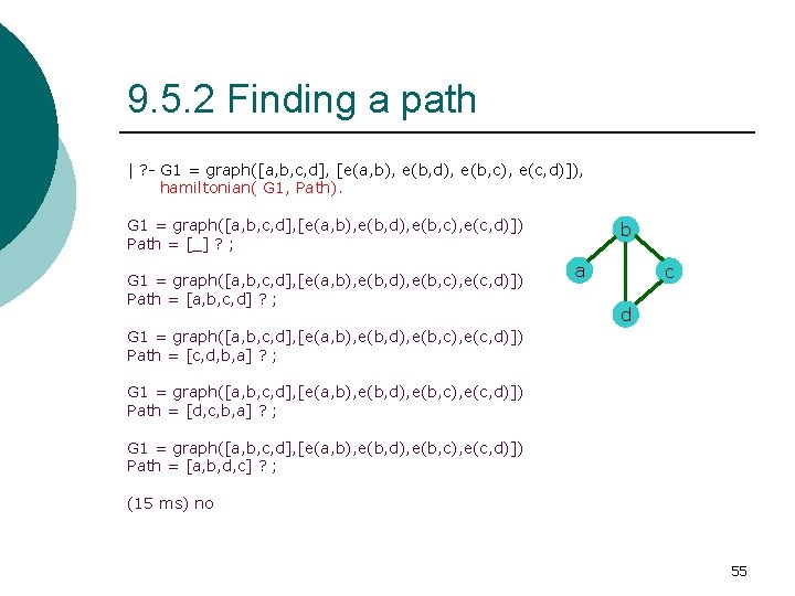
9. 5. 2 Finding a path | ? - G 1 = graph([a, b, c, d], [e(a, b), e(b, d), e(b, c), e(c, d)]), hamiltonian( G 1, Path). G 1 = graph([a, b, c, d], [e(a, b), e(b, d), e(b, c), e(c, d)]) Path = [_] ? ; G 1 = graph([a, b, c, d], [e(a, b), e(b, d), e(b, c), e(c, d)]) Path = [a, b, c, d] ? ; b a c d G 1 = graph([a, b, c, d], [e(a, b), e(b, d), e(b, c), e(c, d)]) Path = [c, d, b, a] ? ; G 1 = graph([a, b, c, d], [e(a, b), e(b, d), e(b, c), e(c, d)]) Path = [d, c, b, a] ? ; G 1 = graph([a, b, c, d], [e(a, b), e(b, d), e(b, c), e(c, d)]) Path = [a, b, d, c] ? ; (15 ms) no 55

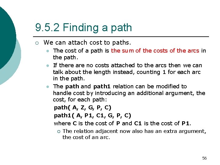
9. 5. 2 Finding a path ¡ We can attach cost to paths. l l l The cost of a path is the sum of the costs of the arcs in the path. If there are no costs attached to the arcs then we can talk about the length instead, counting 1 for each arc in the path. The path and path 1 relation can be modified to handle cost by introducing an additional argument, the cost, for each path: path( A, Z, G, P, C) path 1( A, P 1, C 1, G, P, C) where C is the cost of P and C 1 is the cost of P 1. ¡ The relation adjacent now also has an extra argument, the cost of an arc. 56

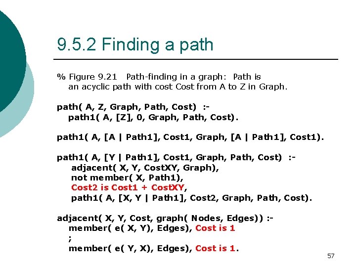
9. 5. 2 Finding a path % Figure 9. 21 Path-finding in a graph: Path is an acyclic path with cost Cost from A to Z in Graph. path( A, Z, Graph, Path, Cost) : path 1( A, [Z], 0, Graph, Path, Cost). path 1( A, [A | Path 1], Cost 1, Graph, [A | Path 1], Cost 1). path 1( A, [Y | Path 1], Cost 1, Graph, Path, Cost) : adjacent( X, Y, Cost. XY, Graph), not member( X, Path 1), Cost 2 is Cost 1 + Cost. XY, path 1( A, [X, Y | Path 1], Cost 2, Graph, Path, Cost). adjacent( X, Y, Cost, graph( Nodes, Edges)) : member( e( X, Y), Edges), Cost is 1 ; member( e( Y, X), Edges), Cost is 1. 57

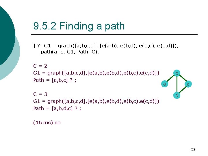
9. 5. 2 Finding a path | ? - G 1 = graph([a, b, c, d], [e(a, b), e(b, d), e(b, c), e(c, d)]), path(a, c, G 1, Path, C). C=2 G 1 = graph([a, b, c, d], [e(a, b), e(b, d), e(b, c), e(c, d)]) Path = [a, b, c] ? ; C=3 G 1 = graph([a, b, c, d], [e(a, b), e(b, d), e(b, c), e(c, d)]) Path = [a, b, d, c] ? ; b a c d (16 ms) no 58

9. 5. 2 Finding a path ¡ We can fine the minimum cost path: | ? - G 1 = graph([a, b, c, d], [e(a, b), e(b, d), e(b, c), e(c, d)]), path(a, c, G 1, Min. Path, Min. Cost), not(( path( a, c, G 1, _, Cost), Cost < Min. Cost)). G 1 = graph([a, b, c, d], [e(a, b), e(b, d), e(b, c), e(c, d)]) Min. Cost = 2 b Min. Path = [a, b, c] ? ; a no c d 59

9. 5. 2 Finding a path ¡ We can fine the maximum cost path: | ? - G 1 = graph([a, b, c, d], [e(a, b), e(b, d), e(b, c), e(c, d)]), path(a, c, G 1, Max. Path, Max. Cost), not(( path( a, c, G 1, _, Cost), Cost > Max. Cost)). G 1 = graph([a, b, c, d], [e(a, b), e(b, d), e(b, c), e(c, d)]) Max. Cost = 3 b Max. Path = [a, b, d, c] ? ; a no c d 60

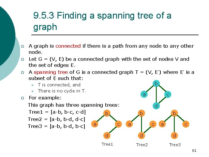
9. 5. 3 Finding a spanning tree of a graph ¡ ¡ ¡ A graph is connected if there is a path from any node to any other node. Let G = (V, E) be a connected graph with the set of nodes V and the set of edges E. A spanning tree of G is a connected graph T = (V, E’) where E’ is a subset of E such that: l l ¡ b T is connected, and There is no cycle in T. For example: This graph has three spanning trees: Tree 1 = [a-b, b-c, c-d] b Tree 2 = [a-b, b-d, d-c] a c Tree 3 = [a-b, b-d, b-c] a c d b a b c a c d d d Tree 1 Tree 2 Tree 3 61

9. 5. 3 Finding a spanning tree of a graph ¡ ¡ ¡ In the edge list of a spanning tree, we can pick any node in such a list as the root of a tree. Spanning trees are of interest in communication problems because they provide, with the minimum number of communication lines, a path between any pair of nodes. Define a procedure stree( G, T) where T is a spanning tree of G. l l l We assume that G is connected. Start with the empty set of edges and gradually add new edges from G, taking care that a cycle is never created, until no more edge can be added because it would create a cycle. The resulting set of edges defines a spanning tree. 62

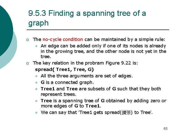
9. 5. 3 Finding a spanning tree of a graph ¡ ¡ The no-cycle condition can be maintained by a simple rule: l An edge can be added only if one of its nodes is already in the growing tree, and the other node is not yet in the tree. The key relation in the probram Figure 9. 22 is: spread( Tree 1, Tree, G) l All the three arguments are set of edges. l G is a connected graph. l Tree 1 and Tree are subsets of G such that they both represent trees. l Tree is a spanning tree of G obtained by adding zero or more edges of G to Tree 1. l We can say that ‘Tree 1 gets spread(擴張) to Tree’. 63

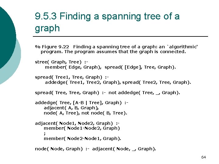
9. 5. 3 Finding a spanning tree of a graph % Figure 9. 22 Finding a spanning tree of a graph: an `algorithmic' program. The program assumes that the graph is connected. stree( Graph, Tree) : member( Edge, Graph), spread( [Edge], Tree, Graph). spread( Tree 1, Tree, Graph) : addedge( Tree 1, Tree 2, Graph), spread( Tree 2, Tree, Graph). spread( Tree, Graph) : - not addedge( Tree, _, Graph). addedge( Tree, [A-B | Tree], Graph) : adjacent( A, B, Graph), node( A, Tree), not node( B, Tree). adjacent( Node 1, Node 2, Graph) : member( Node 1 -Node 2, Graph) ; member( Node 2 -Node 1, Graph). node( Node, Graph) : - adjacent( Node, _, Graph). 64

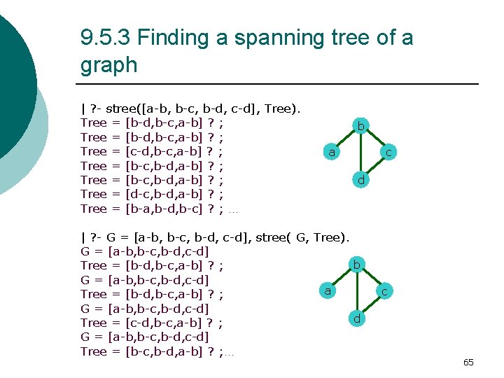
9. 5. 3 Finding a spanning tree of a graph | ? - stree([a-b, b-c, b-d, c-d], Tree). Tree = [b-d, b-c, a-b] ? ; Tree = [c-d, b-c, a-b] ? ; Tree = [b-c, b-d, a-b] ? ; Tree = [d-c, b-d, a-b] ? ; Tree = [b-a, b-d, b-c] ? ; … b a c d | ? - G = [a-b, b-c, b-d, c-d], stree( G, Tree). G = [a-b, b-c, b-d, c-d] b Tree = [b-d, b-c, a-b] ? ; G = [a-b, b-c, b-d, c-d] a Tree = [b-d, b-c, a-b] ? ; G = [a-b, b-c, b-d, c-d] d Tree = [c-d, b-c, a-b] ? ; G = [a-b, b-c, b-d, c-d] Tree = [b-c, b-d, a-b] ? ; … c 65

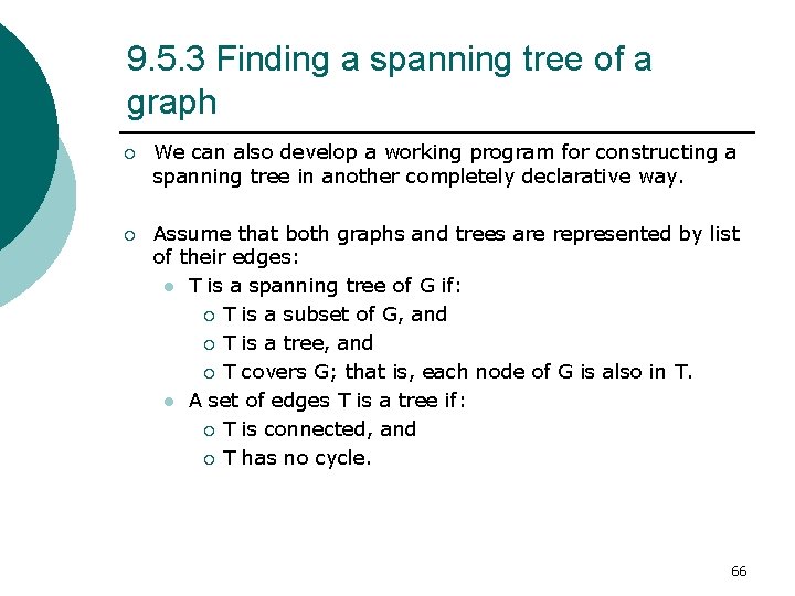
9. 5. 3 Finding a spanning tree of a graph ¡ We can also develop a working program for constructing a spanning tree in another completely declarative way. ¡ Assume that both graphs and trees are represented by list of their edges: l T is a spanning tree of G if: ¡ T is a subset of G, and ¡ T is a tree, and ¡ T covers G; that is, each node of G is also in T. l A set of edges T is a tree if: ¡ T is connected, and ¡ T has no cycle. 66

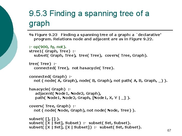
9. 5. 3 Finding a spanning tree of a graph % Figure 9. 23 Finding a spanning tree of a graph: a `declarative' program. Relations node and adjacent are as in Figure 9. 22. : - op(900, fy, not). stree 1( Graph, Tree) : subset( Graph, Tree), tree( Tree), covers( Tree, Graph). tree( Tree) : connected( Tree), not hasacycle( Tree). connected( Graph) : not ( node( A, Graph), node( B, Graph), not path( A, B, Graph, _) ). hasacycle( Graph) : adjacent( Node 1, Node 2, Graph), path( Node 1, Node 2, Graph, [Node 1, X, Y | _] ). covers( Tree, Graph) : not ( node( Node, Graph), not node( Node, Tree) ). subset( [], [] ). subset( [X | Set], Subset) : - subset( Set, Subset). subset( [X | Set], [X | Subset]) : - subset( Set, Subset). 67

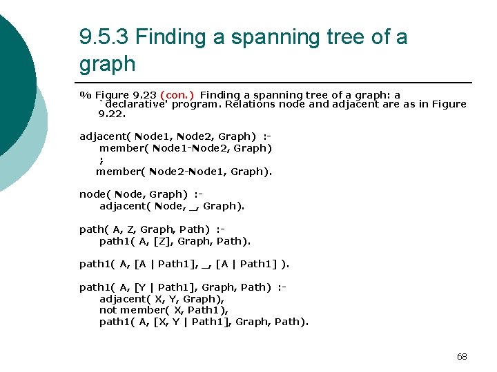
9. 5. 3 Finding a spanning tree of a graph % Figure 9. 23 (con. ) Finding a spanning tree of a graph: a `declarative' program. Relations node and adjacent are as in Figure 9. 22. adjacent( Node 1, Node 2, Graph) : member( Node 1 -Node 2, Graph) ; member( Node 2 -Node 1, Graph). node( Node, Graph) : adjacent( Node, _, Graph). path( A, Z, Graph, Path) : path 1( A, [Z], Graph, Path). path 1( A, [A | Path 1], _, [A | Path 1] ). path 1( A, [Y | Path 1], Graph, Path) : adjacent( X, Y, Graph), not member( X, Path 1), path 1( A, [X, Y | Path 1], Graph, Path). 68

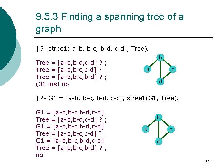
9. 5. 3 Finding a spanning tree of a graph | ? - stree 1([a-b, b-c, b-d, c-d], Tree). Tree = [a-b, b-d, c-d] ? ; Tree = [a-b, b-c, b-d] ? ; (31 ms) no b a c d | ? - G 1 = [a-b, b-c, b-d, c-d], stree 1(G 1, Tree). G 1 = [a-b, b-c, b-d, c-d] Tree = [a-b, b-d, c-d] ? ; G 1 = [a-b, b-c, b-d, c-d] Tree = [a-b, b-c, b-d] ? ; no b a c d 69

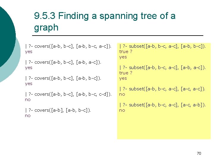
9. 5. 3 Finding a spanning tree of a graph | ? - covers([a-b, b-c], [a-b, b-c, a-c]). yes | ? - covers([a-b, b-c], [a-b, b-c]). yes | ? - covers([a-b, b-c], [a-b, b-c, c-d]). no | ? - covers([a-b], [a-b, b-c]). no | ? - subset([a-b, b-c, a-c], [a-b, b-c]). true ? yes | ? - subset([a-b, b-c, a-c], [a-b, a-c]). true ? yes | ? - subset([a-b, b-c, a-c], [a-c, a-c]). no | ? - subset([a-b, b-c, a-c], [a-c, a-b]). no 70