Part 1 The Prolog Language Chapter 8 Programming

Part 1 The Prolog Language Chapter 8 Programming Style and Technique 1

8. 1 General principles of good programming ¡ What is a good program? l Generally accepted criteria include the following: Correctness ¡ User-friendliness ¡ Efficiency ¡ Readability ¡ Modifiability ¡ Robustness ¡ Documentation ¡ 2

8. 2 How to think about Prolog programs ¡ ¡ During the process of developing a solution we have to find ideas for reducing problems to one or more easier subproblems. How do we find proper subproblems? l l l Use of recursion (Section 8. 2. 1) Generalization (Section 8. 2. 2) Using pictures (Section 8. 2. 3) 3

8. 2. 1 Use of recursion ¡ The principle here is to split the problem into two cases: (1) trivial, or boundary cases; (2) general cases where the solution is constructed(建構) from solutions of (simpler) versions of the original program itself. ¡ An example: l Processing a list of items so that each item is transformed by the same transformation rule. maplist( List, F, New. List) where List is an original list, F is a transformation rule and New. List is the list of all transformed items. 4

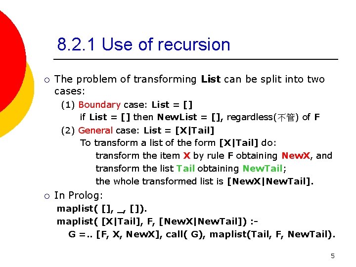
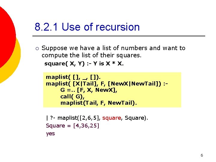
8. 2. 1 Use of recursion ¡ The problem of transforming List can be split into two cases: (1) Boundary case: List = [] if List = [] then New. List = [], regardless(不管) of F (2) General case: List = [X|Tail] To transform a list of the form [X|Tail] do: transform the item X by rule F obtaining New. X, and transform the list Tail obtaining New. Tail; the whole transformed list is [New. X|New. Tail]. ¡ In Prolog: maplist( [], _, []). maplist( [X|Tail], F, [New. X|New. Tail]) : G =. . [F, X, New. X], call( G), maplist(Tail, F, New. Tail). 5

8. 2. 1 Use of recursion ¡ Suppose we have a list of numbers and want to compute the list of their squares. square( X, Y) : - Y is X * X. maplist( [], _, []). maplist( [X|Tail], F, [New. X|New. Tail]) : G =. . [F, X, New. X], call( G), maplist(Tail, F, New. Tail). | ? - maplist([2, 6, 5], square, Square). Square = [4, 36, 25] yes 6

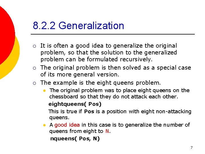
8. 2. 2 Generalization ¡ ¡ ¡ It is often a good idea to generalize the original problem, so that the solution to the generalized problem can be formulated recursively. The original problem is then solved as a special case of its more general version. The example is the eight queens problem. l l The original problem was to place eight queens on the chessboard so that they do not attack each other. eightqueens( Pos) This is true if Pos is a position with eight non-attacking queens. A good idea in this case is to generalize the number of queens from eight to N. nqueens( Pos, N) 7

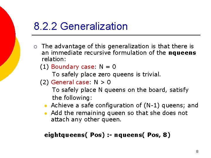
8. 2. 2 Generalization ¡ The advantage of this generalization is that there is an immediate recursive formulation of the nqueens relation: (1) Boundary case: N = 0 To safely place zero queens is trivial. (2) General case: N > 0 To safely place N queens on the board, satisfy the following: l Achieve a safe configuration of (N-1) queens; and l Add the remaining queen so that she does not attach any other queen. eightqueens( Pos) : - nqueens( Pos, 8) 8

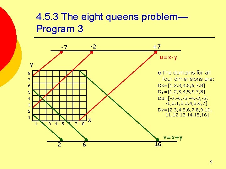
4. 5. 3 The eight queens problem— Program 3 -2 -7 +7 u=x-y y ¡ The domains for all four dimensions are: 8 7 6 5 4 ● 3 2 1 1 2 3 4 5 6 7 8 x Dx=[1, 2, 3, 4, 5, 6, 7, 8] Dy=[1, 2, 3, 4, 5, 6, 7, 8] Du=[-7, -6, -5, -4, -3, -2, -1, 0, 1, 2, 3, 4, 5, 6, 7] Dv=[2, 3, 4, 5, 6, 7, 8, 9, 10, 11, 12, 13, 14, 15, 16] v=x+y 2 6 16 9

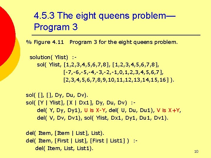
4. 5. 3 The eight queens problem— Program 3 % Figure 4. 11 Program 3 for the eight queens problem. solution( Ylist) : sol( Ylist, [1, 2, 3, 4, 5, 6, 7, 8], [-7, -6, -5, -4, -3, -2, -1, 0, 1, 2, 3, 4, 5, 6, 7], [2, 3, 4, 5, 6, 7, 8, 9, 10, 11, 12, 13, 14, 15, 16] ). sol( [], Dy, Du, Dv). sol( [Y | Ylist], [X | Dx 1], Dy, Du, Dv) : del( Y, Dy 1), U is X-Y, del( U, Du 1), V is X+Y, del( V, Dv 1), sol( Ylist, Dx 1, Dy 1, Du 1, Dv 1). del( Item, [Item | List], List). del( Item, [First | List], [First | List 1] ) : del( Item, List 1). 10

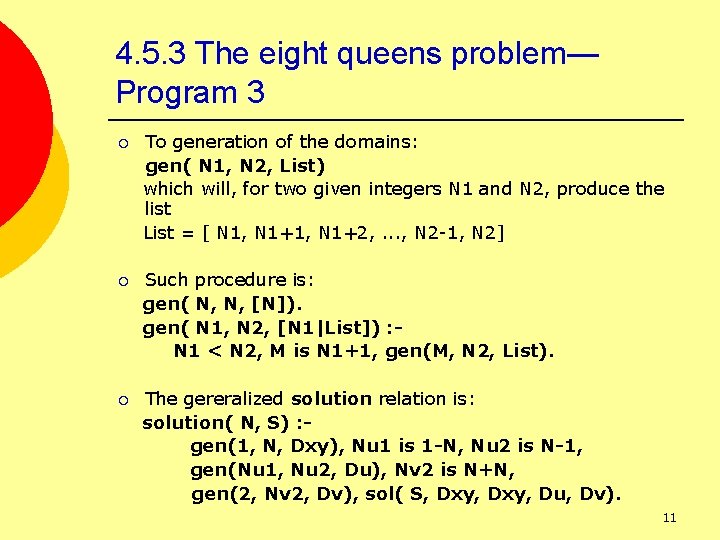
4. 5. 3 The eight queens problem— Program 3 ¡ To generation of the domains: gen( N 1, N 2, List) which will, for two given integers N 1 and N 2, produce the list List = [ N 1, N 1+2, . . . , N 2 -1, N 2] ¡ Such procedure is: gen( N, N, [N]). gen( N 1, N 2, [N 1|List]) : N 1 < N 2, M is N 1+1, gen(M, N 2, List). ¡ The gereralized solution relation is: solution( N, S) : gen(1, N, Dxy), Nu 1 is 1 -N, Nu 2 is N-1, gen(Nu 1, Nu 2, Du), Nv 2 is N+N, gen(2, Nv 2, Dv), sol( S, Dxy, Du, Dv). 11

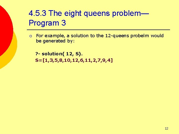
4. 5. 3 The eight queens problem— Program 3 ¡ For example, a solution to the 12 -queens probelm would be generated by: ? - solution( 12, S). S=[1, 3, 5, 8, 10, 12, 6, 11, 2, 7, 9, 4] 12

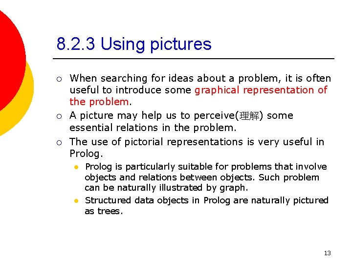
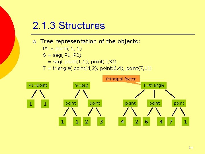
8. 2. 3 Using pictures ¡ ¡ ¡ When searching for ideas about a problem, it is often useful to introduce some graphical representation of the problem. A picture may help us to perceive(理解) some essential relations in the problem. The use of pictorial representations is very useful in Prolog. l l Prolog is particularly suitable for problems that involve objects and relations between objects. Such problem can be naturally illustrated by graph. Structured data objects in Prolog are naturally pictured as trees. 13

2. 1. 3 Structures ¡ Tree representation of the objects: P 1 = point( 1, 1) S = seg( P 1, P 2) = seg( point(1, 1), point(2, 3)) T = triangle( point(4, 2), point(6, 4), point(7, 1)) Principal factor P 1=point 1 S=seg 1 point 1 1 T=triangle point 2 3 point 4 2 point 6 4 point 7 1 14

8. 3 Programming style ¡ The purpose of conforming to some stylistic(文體的) conventions(慣例) is: l l To reduce the danger of programming errors; and To produce programs that are ¡ ¡ readable and easy to understand easy to debug and to modify 15

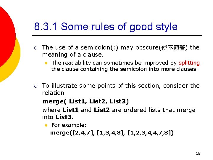
8. 3. 1 Some rules of good style ¡ ¡ Program clauses should be short. Procedures should be short because long procedures are hard to understand. Mnemonic(有助記憶的) names for procedures and variables should be used. The layout(版面編排) of programs is important. l l l ¡ Spacing, blank lines and indentation(縮排) should be consistently used for the sake(目的) of readability. Clauses about the same procedure should be clustered together. There should be blank lines between clauses. Stylistic conventions of this kind may vary from program to program. However, it is important that the same conventions are used consistently throughout the whole program. 16

8. 3. 1 Some rules of good style ¡ The cut operator should be used with care. l l ¡ The not procedure can also lead to surprising behavior, as it is related to cut. l ¡ Cut should not be used if it can be easily avoided. It is better to use ‘green cuts’ rather than ‘red cuts’. If there is a dilemma(兩難的選擇) between not and cut, the former is perhaps better than some obscure(模糊的 ) construct with cut. Program modification by assert and retract can grossly(非常地) degrade the transparency (降低透明度 ) of the program’s behavior. l In particular, the same program will answer the same question differently at different times. 17

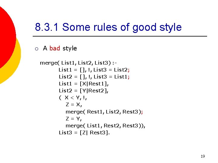
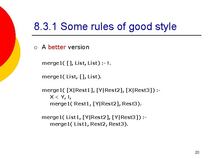
8. 3. 1 Some rules of good style ¡ The use of a semicolon(; ) may obscure(使不顯著) the meaning of a clause. l ¡ The readability can sometimes be improved by splitting the clause containing the semicolon into more clauses. To illustrate some points of this section, consider the relation merge( List 1, List 2, List 3) where List 1 and List 2 are ordered lists that merge into List 3. l For example: merge([2, 4, 7], [1, 3, 4, 8], [1, 2, 3, 4, 4, 7, 8]) 18

8. 3. 1 Some rules of good style ¡ A bad style merge( List 1, List 2, List 3) : List 1 = [], !, List 3 = List 2; List 2 = [], !, List 3 = List 1; List 1 = [X|Rest 1], List 2 = [Y|Rest 2], ( X < Y, !, Z = X, merge( Rest 1, List 2, Rest 3); Z = Y, merge( List 1, Rest 2, Rest 3)), List 3 = [Z| Rest 3]. 19

8. 3. 1 Some rules of good style ¡ A better version merge 1( [], List) : - !. merge 1( List, [], List). merge 1( [X|Rest 1], [Y|Rest 2], [X|Rest 3]) : X < Y, !, merge 1( Rest 1, [Y|Rest 2], Rest 3). merge 1( List 1, [Y|Rest 2], [Y|Rest 3]) : merge 1( List 1, Rest 2, Rest 3). 20

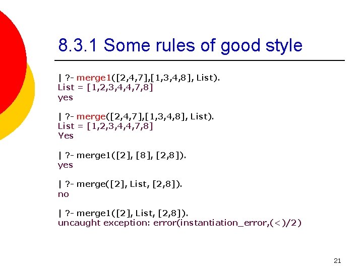
8. 3. 1 Some rules of good style | ? - merge 1([2, 4, 7], [1, 3, 4, 8], List). List = [1, 2, 3, 4, 4, 7, 8] yes | ? - merge([2, 4, 7], [1, 3, 4, 8], List). List = [1, 2, 3, 4, 4, 7, 8] Yes | ? - merge 1([2], [8], [2, 8]). yes | ? - merge([2], List, [2, 8]). no | ? - merge 1([2], List, [2, 8]). uncaught exception: error(instantiation_error, (<)/2) 21

8. 3. 2 Tabular organization of long procedures ¡ ¡ ¡ Long procedures are acceptable if they have some uniform structure. Such a form is a set of facts when a relation is effectively defined in the tabular(列表的) form. The advantages of such an organization of a long procedure are: l l l Its structure is easily understood. Incrementability: it can be refined by simply adding new facts. It is easy to check and correct or modify by simply replacing some fact independently of other facts. 22

8. 3. 3 Commenting ¡ ¡ The main purpose of comments is to enable the user to use the program, to understand it and to possibly modify it. Long passages(一段) of comments should precede the code they refer to, while short comments should be interspersed with the code itself. 23

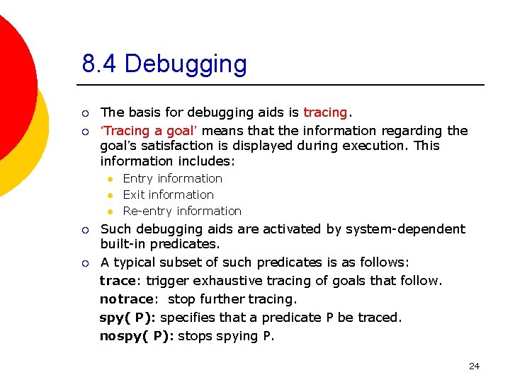
8. 4 Debugging ¡ ¡ The basis for debugging aids is tracing. ‘Tracing a goal’ means that the information regarding the goal’s satisfaction is displayed during execution. This information includes: l l l ¡ ¡ Entry information Exit information Re-entry information Such debugging aids are activated by system-dependent built-in predicates. A typical subset of such predicates is as follows: trace: trigger exhaustive tracing of goals that follow. notrace: stop further tracing. spy( P): specifies that a predicate P be traced. nospy( P): stops spying P. 24

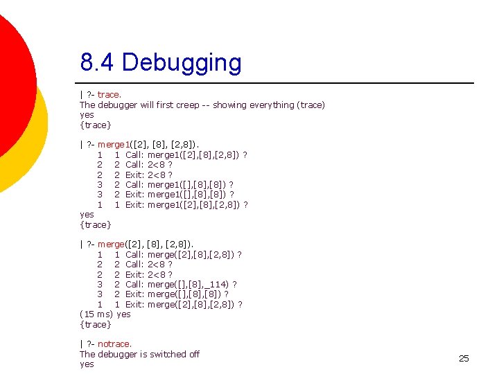
8. 4 Debugging | ? - trace. The debugger will first creep -- showing everything (trace) yes {trace} | ? - merge 1([2], [8], [2, 8]). 1 1 Call: merge 1([2], [8], [2, 8]) ? 2 2 Call: 2<8 ? 2 2 Exit: 2<8 ? 3 2 Call: merge 1([], [8]) ? 3 2 Exit: merge 1([], [8]) ? 1 1 Exit: merge 1([2], [8], [2, 8]) ? yes {trace} | ? - merge([2], [8], [2, 8]). 1 1 Call: merge([2], [8], [2, 8]) ? 2 2 Call: 2<8 ? 2 2 Exit: 2<8 ? 3 2 Call: merge([], [8], _114) ? 3 2 Exit: merge([], [8]) ? 1 1 Exit: merge([2], [8], [2, 8]) ? (15 ms) yes {trace} | ? - notrace. The debugger is switched off yes 25

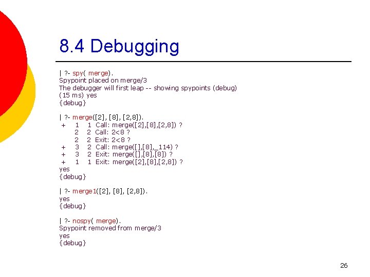
8. 4 Debugging | ? - spy( merge). Spypoint placed on merge/3 The debugger will first leap -- showing spypoints (debug) (15 ms) yes {debug} | ? - merge([2], [8], [2, 8]). + 1 1 Call: merge([2], [8], [2, 8]) ? 2 2 Call: 2<8 ? 2 2 Exit: 2<8 ? + 3 2 Call: merge([], [8], _114) ? + 3 2 Exit: merge([], [8]) ? + 1 1 Exit: merge([2], [8], [2, 8]) ? yes {debug} | ? - merge 1([2], [8], [2, 8]). yes {debug} | ? - nospy( merge). Spypoint removed from merge/3 yes {debug} 26

8. 5 Improving efficiency ¡ ¡ Ideas for improving the efficiency of a program usually come from a deeper understanding of the problem. A more efficient algorithm can result from improvements of two kinds: l l Improving search efficiency by avoiding unnecessary backtracking and stopping the execution of useless alternatives as soon as possible. Using more suitable data structures to represent objects in the program, so that operations on objects can be implemented more efficiently. 27

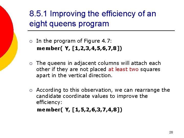
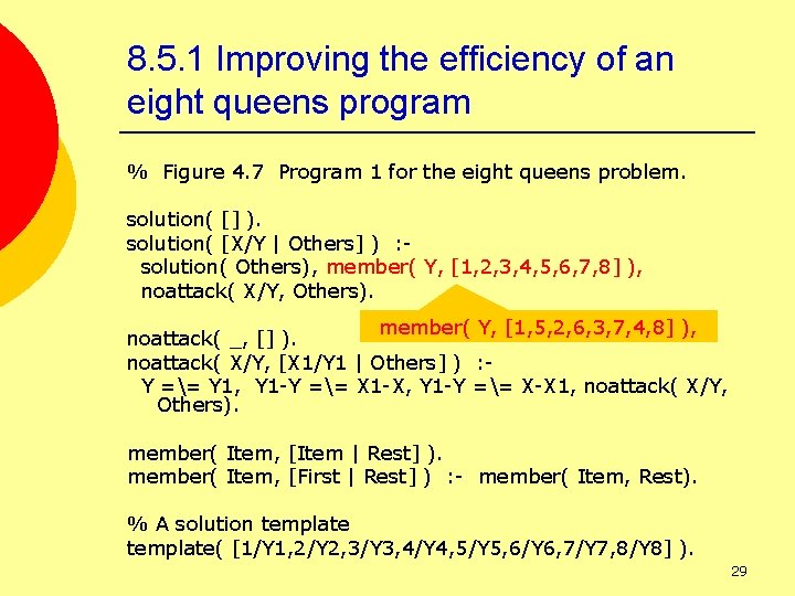
8. 5. 1 Improving the efficiency of an eight queens program ¡ In the program of Figure 4. 7: member( Y, [1, 2, 3, 4, 5, 6, 7, 8]) ¡ The queens in adjacent columns will attach each other if they are not placed at least two squares apart in the vertical direction. ¡ According to this observation, we can rearrange the candidate coordinate values to improve the efficiency: member( Y, [1, 5, 2, 6, 3, 7, 4, 8]) 28

8. 5. 1 Improving the efficiency of an eight queens program % Figure 4. 7 Program 1 for the eight queens problem. solution( [] ). solution( [X/Y | Others] ) : solution( Others), member( Y, [1, 2, 3, 4, 5, 6, 7, 8] ), noattack( X/Y, Others). member( Y, [1, 5, 2, 6, 3, 7, 4, 8] ), noattack( _, [] ). noattack( X/Y, [X 1/Y 1 | Others] ) : Y == Y 1, Y 1 -Y == X 1 -X, Y 1 -Y == X-X 1, noattack( X/Y, Others). member( Item, [Item | Rest] ). member( Item, [First | Rest] ) : - member( Item, Rest). % A solution template( [1/Y 1, 2/Y 2, 3/Y 3, 4/Y 4, 5/Y 5, 6/Y 6, 7/Y 7, 8/Y 8] ). 29

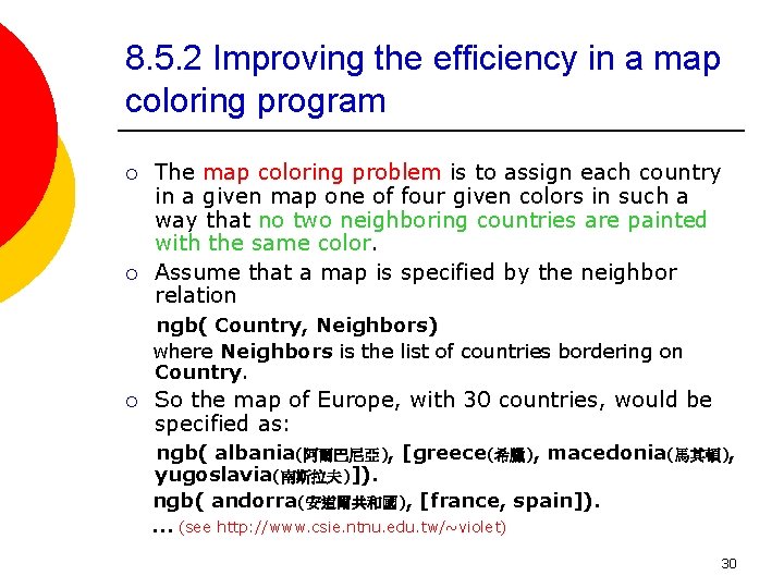
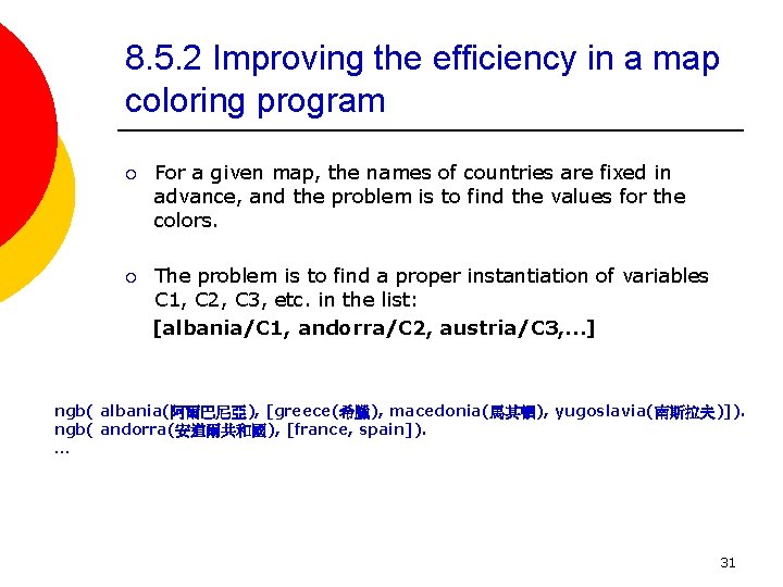
8. 5. 2 Improving the efficiency in a map coloring program ¡ ¡ The map coloring problem is to assign each country in a given map one of four given colors in such a way that no two neighboring countries are painted with the same color. Assume that a map is specified by the neighbor relation ngb( Country, Neighbors) where Neighbors is the list of countries bordering on Country. ¡ So the map of Europe, with 30 countries, would be specified as: ngb( albania(阿爾巴尼亞), [greece(希臘), macedonia(馬其頓), yugoslavia(南斯拉夫)]). ngb( andorra(安道爾共和國), [france, spain]). … (see http: //www. csie. ntnu. edu. tw/~violet) 30

8. 5. 2 Improving the efficiency in a map coloring program ¡ For a given map, the names of countries are fixed in advance, and the problem is to find the values for the colors. ¡ The problem is to find a proper instantiation of variables C 1, C 2, C 3, etc. in the list: [albania/C 1, andorra/C 2, austria/C 3, …] ngb( albania(阿爾巴尼亞), [greece(希臘), macedonia(馬其頓), yugoslavia(南斯拉夫)]). ngb( andorra(安道爾共和國), [france, spain]). … 31

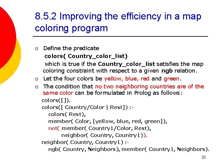
8. 5. 2 Improving the efficiency in a map coloring program ¡ ¡ ¡ Define the predicate colors( Country_color_list) which is true if the Country_color_list satisfies the map coloring constraint with respect to a given ngb relation. Let the four colors be yellow, blue, red and green. The condition that no two neighboring countries are of the same color can be formulated in Prolog as follows: colors([]). colors([ Country/Color | Rest]) : colors( Rest), member( Color, [yellow, blue, red, green]), not( member( Country 1/Color, Rest), neighbor( Country, Country 1)). neighbor( Country, Country 1) : ngb( Country, Neighbors), member( Country 1, Neighbors). 32

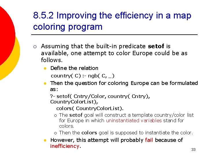
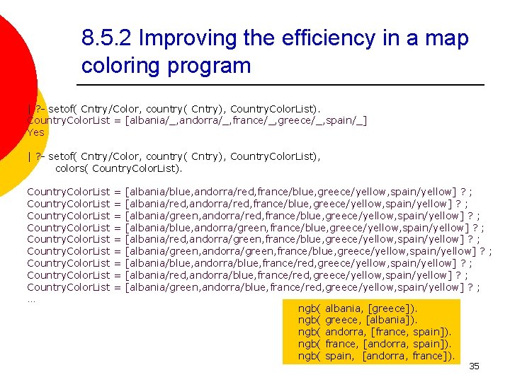
8. 5. 2 Improving the efficiency in a map coloring program ¡ Assuming that the built-in predicate setof is available, one attempt to color Europe could be as follows. l Define the relation country( C) : - ngb( C, _) l Then the question for coloring Europe can be formulated as: ? - setof( Cntry/Color, country( Cntry), Country. Color. List), colors( Country. Color. List). ¡ The setof goal will construct a template country/color list for Europe in which uninstantiated variables stand for colors. ¡ Then the colors goal is supposed to instantiate the color. l However, this attempt will probably fail because of inefficiency. 33

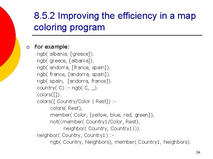
8. 5. 2 Improving the efficiency in a map coloring program ¡ For example: ngb( albania, [greece]). ngb( greece, [albania]). ngb( andorra, [france, spain]). ngb( france, [andorra, spain]). ngb( spain, [andorra, france]). country( C) : - ngb( C, _). colors([]). colors([ Country/Color | Rest]) : colors( Rest), member( Color, [yellow, blue, red, green]), not((member( Country 1/Color, Rest), neighbor( Country, Country 1))). neighbor( Country, Country 1) : ngb( Country, Neighbors), member( Country 1, Neighbors). 34

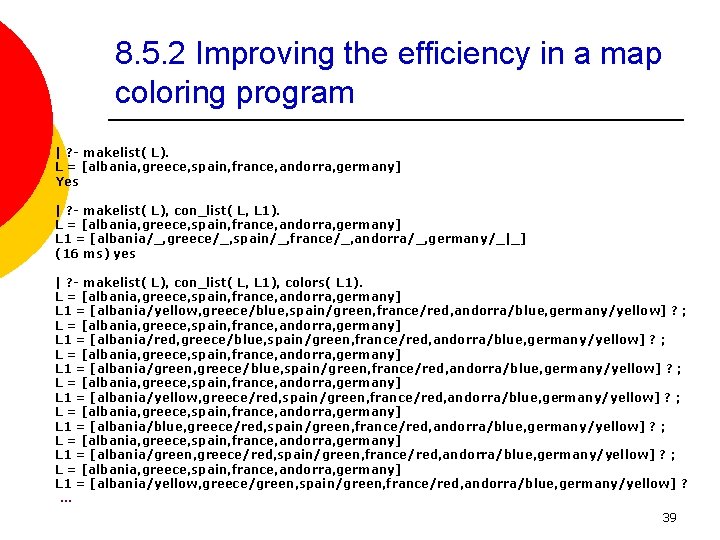
8. 5. 2 Improving the efficiency in a map coloring program | ? - setof( Cntry/Color, country( Cntry), Country. Color. List). Country. Color. List = [albania/_, andorra/_, france/_, greece/_, spain/_] Yes | ? - setof( Cntry/Color, country( Cntry), Country. Color. List), colors( Country. Color. List). Country. Color. List Country. Color. List … = = = = = [albania/blue, andorra/red, france/blue, greece/yellow, spain/yellow] ? ; [albania/red, andorra/red, france/blue, greece/yellow, spain/yellow] ? ; [albania/green, andorra/red, france/blue, greece/yellow, spain/yellow] ? ; [albania/blue, andorra/green, france/blue, greece/yellow, spain/yellow] ? ; [albania/red, andorra/green, france/blue, greece/yellow, spain/yellow] ? ; [albania/green, andorra/green, france/blue, greece/yellow, spain/yellow] ? ; [albania/blue, andorra/blue, france/red, greece/yellow, spain/yellow] ? ; [albania/red, andorra/blue, france/red, greece/yellow, spain/yellow] ? ; [albania/green, andorra/blue, france/red, greece/yellow, spain/yellow] ? ; ngb( ngb( albania, [greece]). greece, [albania]). andorra, [france, spain]). france, [andorra, spain]). spain, [andorra, france]). 35

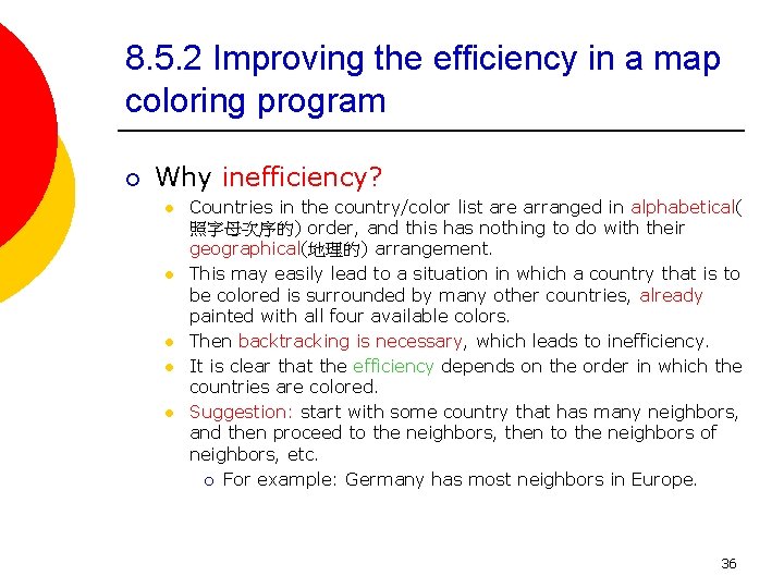
8. 5. 2 Improving the efficiency in a map coloring program ¡ Why inefficiency? l l l Countries in the country/color list are arranged in alphabetical( 照字母次序的) order, and this has nothing to do with their geographical(地理的) arrangement. This may easily lead to a situation in which a country that is to be colored is surrounded by many other countries, already painted with all four available colors. Then backtracking is necessary, which leads to inefficiency. It is clear that the efficiency depends on the order in which the countries are colored. Suggestion: start with some country that has many neighbors, and then proceed to the neighbors, then to the neighbors of neighbors, etc. ¡ For example: Germany has most neighbors in Europe. 36

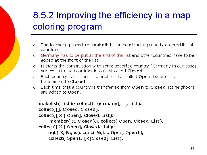
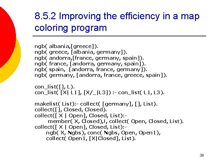
8. 5. 2 Improving the efficiency in a map coloring program ¡ ¡ ¡ The following procedure, makelist, can construct a properly ordered list of countries. Germany has to be put at the end of the list and other countries have to be added at the front of the list. It starts the construction with some specified country (Germany in our case) and collects the countries into a list called Closed. Each country is first put into another list, called Open, before it is transferred to Closed. Each time that a country is transferred from Open to Closed, its neighbors are added to Open. makelist( List): - collect( [germany], [], List). collect([], Closed). collect([ X | Open], Closed, List): member( X, Closed), !, collect( Open, Closed, List). collect([ X | Open], Closed, List): ngb( X, Ngbs), conc( Ngbs, Open 1), collect( Open 1, [X|Closed], List). 37

8. 5. 2 Improving the efficiency in a map coloring program ngb( ngb( albania, [greece]). greece, [albania, germany]). andorra, [france, germany, spain]). france, [andorra, germany, spain]). spain, [andorra, france, germany]). germany, [andorra, france, greece, spain]). con_list([], L). con_list( [X| L 1], [X/_|L 3]) : - con_list( L 1, L 3). makelist( List): - collect( [germany], [], List). collect([], Closed). collect([ X | Open], Closed, List): member( X, Closed), !, collect( Open, Closed, List). collect([ X | Open], Closed, List): ngb( X, Ngbs), conc( Ngbs, Open 1), collect( Open 1, [X|Closed], List). 38

8. 5. 2 Improving the efficiency in a map coloring program | ? - makelist( L). L = [albania, greece, spain, france, andorra, germany] Yes | ? - makelist( L), con_list( L, L 1). L = [albania, greece, spain, france, andorra, germany] L 1 = [albania/_, greece/_, spain/_, france/_, andorra/_, germany/_|_] (16 ms) yes | ? - makelist( L), con_list( L, L 1), colors( L 1). L = [albania, greece, spain, france, andorra, germany] L 1 = [albania/yellow, greece/blue, spain/green, france/red, andorra/blue, germany/yellow] ? ; L = [albania, greece, spain, france, andorra, germany] L 1 = [albania/red, greece/blue, spain/green, france/red, andorra/blue, germany/yellow] ? ; L = [albania, greece, spain, france, andorra, germany] L 1 = [albania/green, greece/blue, spain/green, france/red, andorra/blue, germany/yellow] ? ; L = [albania, greece, spain, france, andorra, germany] L 1 = [albania/yellow, greece/red, spain/green, france/red, andorra/blue, germany/yellow] ? ; L = [albania, greece, spain, france, andorra, germany] L 1 = [albania/blue, greece/red, spain/green, france/red, andorra/blue, germany/yellow] ? ; L = [albania, greece, spain, france, andorra, germany] L 1 = [albania/green, greece/red, spain/green, france/red, andorra/blue, germany/yellow] ? ; L = [albania, greece, spain, france, andorra, germany] L 1 = [albania/yellow, greece/green, spain/green, france/red, andorra/blue, germany/yellow] ? … 39

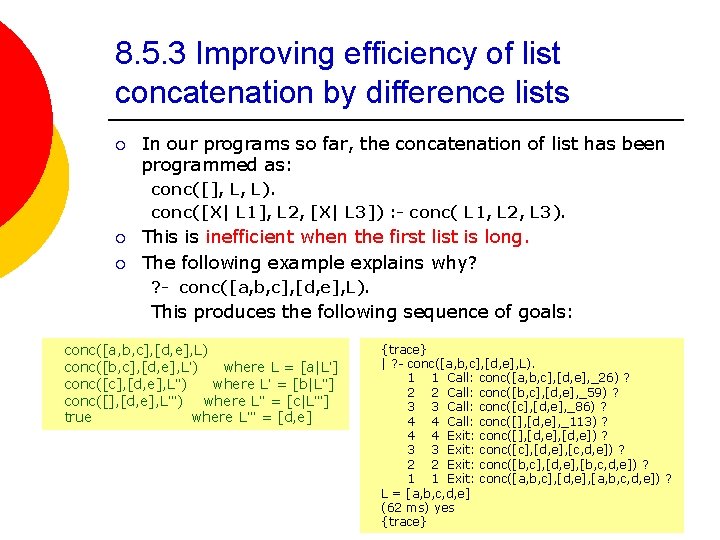
8. 5. 3 Improving efficiency of list concatenation by difference lists ¡ In our programs so far, the concatenation of list has been programmed as: conc([], L, L). conc([X| L 1], L 2, [X| L 3]) : - conc( L 1, L 2, L 3). ¡ ¡ This is inefficient when the first list is long. The following example explains why? ? - conc([a, b, c], [d, e], L). This produces the following sequence of goals: conc([a, b, c], [d, e], L) conc([b, c], [d, e], L’) where L = [a|L’] conc([c], [d, e], L’’) where L’ = [b|L’’] conc([], [d, e], L’’’) where L’’ = [c|L’’’] true where L’’’ = [d, e] {trace} | ? - conc([a, b, c], [d, e], L). 1 1 Call: conc([a, b, c], [d, e], _26) ? 2 2 Call: conc([b, c], [d, e], _59) ? 3 3 Call: conc([c], [d, e], _86) ? 4 4 Call: conc([], [d, e], _113) ? 4 4 Exit: conc([], [d, e]) ? 3 3 Exit: conc([c], [d, e], [c, d, e]) ? 2 2 Exit: conc([b, c], [d, e], [b, c, d, e]) ? 1 1 Exit: conc([a, b, c], [d, e], [a, b, c, d, e]) ? L = [a, b, c, d, e] (62 ms) yes 40 {trace}

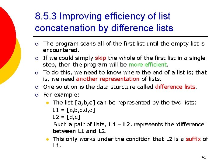
8. 5. 3 Improving efficiency of list concatenation by difference lists ¡ ¡ ¡ The program scans all of the first list until the empty list is encountered. If we could simply skip the whole of the first list in a single step, then the program will be more efficient. To do this, we need to know where the end of a list is; that is, we need another representation of lists. One solution is the data sturcture called difference lists. For example: l The list [a, b, c] can be represented by the two lists: L 1 = [a, b, c, d, e] L 2 = [d, e] l Such a pair of lists, L 1 – L 2, represents the ‘difference’ between L 1 and L 2. This only works under the condition that L 2 is a suffix of L 1. 41

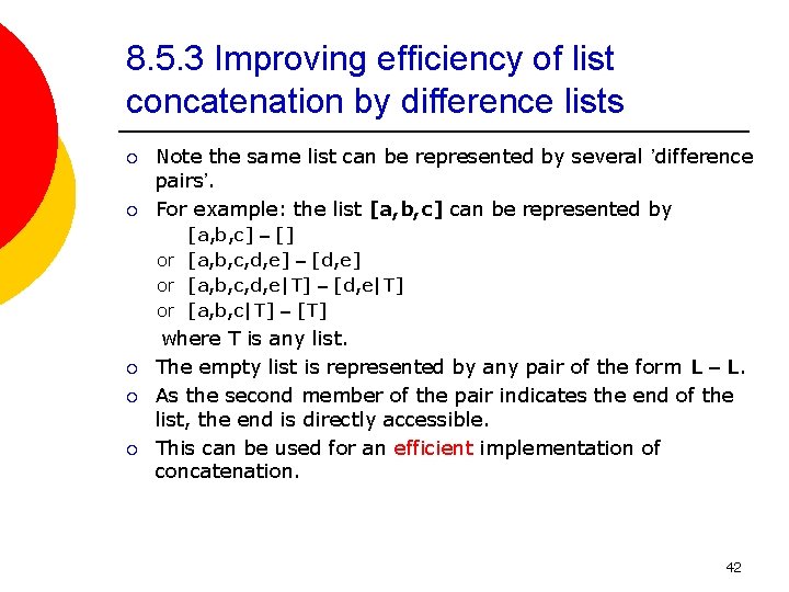
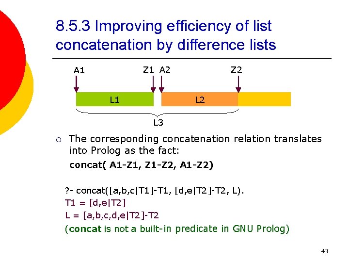
8. 5. 3 Improving efficiency of list concatenation by difference lists ¡ ¡ Note the same list can be represented by several ’difference pairs’. For example: the list [a, b, c] can be represented by [a, b, c] – [] or [a, b, c, d, e] – [d, e] or [a, b, c, d, e|T] – [d, e|T] or [a, b, c|T] – [T] ¡ ¡ ¡ where T is any list. The empty list is represented by any pair of the form L – L. As the second member of the pair indicates the end of the list, the end is directly accessible. This can be used for an efficient implementation of concatenation. 42

8. 5. 3 Improving efficiency of list concatenation by difference lists Z 1 A 2 A 1 L 1 Z 2 L 3 ¡ The corresponding concatenation relation translates into Prolog as the fact: concat( A 1 -Z 1, Z 1 -Z 2, A 1 -Z 2) ? - concat([a, b, c|T 1]-T 1, [d, e|T 2]-T 2, L). T 1 = [d, e|T 2] L = [a, b, c, d, e|T 2]-T 2 (concat is not a built-in predicate in GNU Prolog) 43

8. 5. 4 Last call optimization and accumulators ¡ ¡ ¡ Recursive call normally take up memory space, which is only freed after the return from the call. A large number of nested recursive calls may lead to shortage of memory. In special cases, it is possible to execute nested recursive calls without requiring extra memory. In such a case a recursive procedure has a special form, call tail recursion. A tail-recursive procedure l l It only has one recursive call, and the call appears as the last goal of the last clause in the procedure. The goals preceding the recursive call must be deterministic, so that no backtracking occurs after this last call. 44

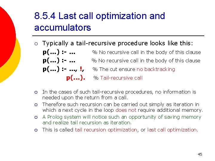
8. 5. 4 Last call optimization and accumulators ¡ ¡ ¡ Typically a tail-recursive procedure looks like this: p(. . . ) : -. . . % No recursive call in the body of this clause p(. . . ) : -. . . , !, % The cut ensure no backtracking p(. . . ). % Tail-recursive call In the cases of such tail-recursive procedures, no information is needed upon the return from a call. Therefore such recursion can be carried out simply as iteration in which a next cycle in the loop does not require additional memory. A Prolog system will notice such an opportunity of saving memory and realize tail recursion as iteration. This is called tail recursion optimization, or last call optimization. 45

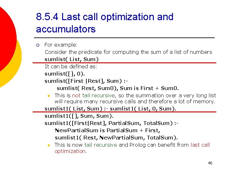
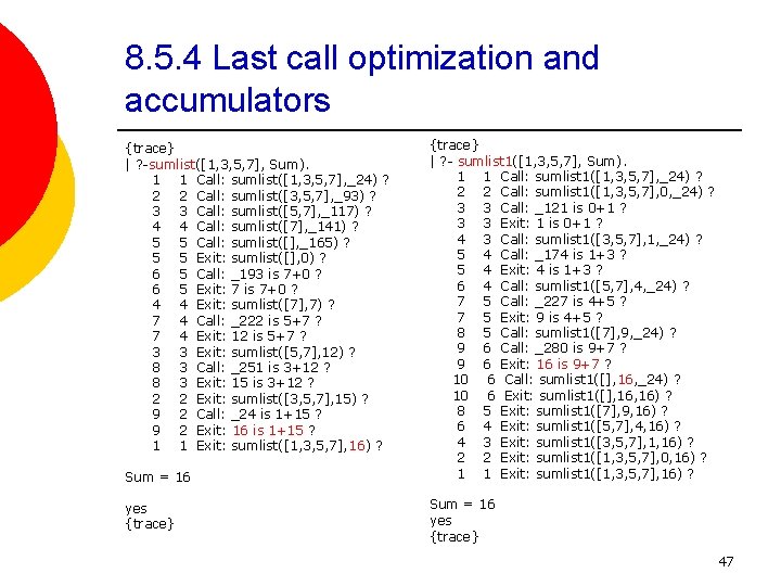
8. 5. 4 Last call optimization and accumulators ¡ For example: Consider the predicate for computing the sum of a list of numbers sumlist( List, Sum) It can be defined as: sumlist([], 0). sumlist([First |Rest], Sum) : sumlist( Rest, Sum 0), Sum is First + Sum 0. l This is not tail recursive, so the summation over a very long list will require many recursive calls and therefore a lot of memory. sumlist 1( List, Sum) : - sumlist 1( List, 0, Sum). sumlist 1([], Sum). sumlist 1([First|Rest], Partial. Sum, Total. Sum) : New. Partial. Sum is Partial. Sum + First, sumlist 1( Rest, New. Partial. Sum, Total. Sum). l This is now tail recursive and Prolog can benefit from last call optimization. 46

8. 5. 4 Last call optimization and accumulators {trace} | ? -sumlist([1, 3, 5, 7], Sum). 1 1 Call: sumlist([1, 3, 5, 7], _24) ? 2 2 Call: sumlist([3, 5, 7], _93) ? 3 3 Call: sumlist([5, 7], _117) ? 4 4 Call: sumlist([7], _141) ? 5 5 Call: sumlist([], _165) ? 5 5 Exit: sumlist([], 0) ? 6 5 Call: _193 is 7+0 ? 6 5 Exit: 7 is 7+0 ? 4 4 Exit: sumlist([7], 7) ? 7 4 Call: _222 is 5+7 ? 7 4 Exit: 12 is 5+7 ? 3 3 Exit: sumlist([5, 7], 12) ? 8 3 Call: _251 is 3+12 ? 8 3 Exit: 15 is 3+12 ? 2 2 Exit: sumlist([3, 5, 7], 15) ? 9 2 Call: _24 is 1+15 ? 9 2 Exit: 16 is 1+15 ? 1 1 Exit: sumlist([1, 3, 5, 7], 16) ? Sum = 16 yes {trace} | ? - sumlist 1([1, 3, 5, 7], Sum). 1 1 Call: sumlist 1([1, 3, 5, 7], _24) ? 2 2 Call: sumlist 1([1, 3, 5, 7], 0, _24) ? 3 3 Call: _121 is 0+1 ? 3 3 Exit: 1 is 0+1 ? 4 3 Call: sumlist 1([3, 5, 7], 1, _24) ? 5 4 Call: _174 is 1+3 ? 5 4 Exit: 4 is 1+3 ? 6 4 Call: sumlist 1([5, 7], 4, _24) ? 7 5 Call: _227 is 4+5 ? 7 5 Exit: 9 is 4+5 ? 8 5 Call: sumlist 1([7], 9, _24) ? 9 6 Call: _280 is 9+7 ? 9 6 Exit: 16 is 9+7 ? 10 6 Call: sumlist 1([], 16, _24) ? 10 6 Exit: sumlist 1([], 16) ? 8 5 Exit: sumlist 1([7], 9, 16) ? 6 4 Exit: sumlist 1([5, 7], 4, 16) ? 4 3 Exit: sumlist 1([3, 5, 7], 1, 16) ? 2 2 Exit: sumlist 1([1, 3, 5, 7], 0, 16) ? 1 1 Exit: sumlist 1([1, 3, 5, 7], 16) ? Sum = 16 yes {trace} 47

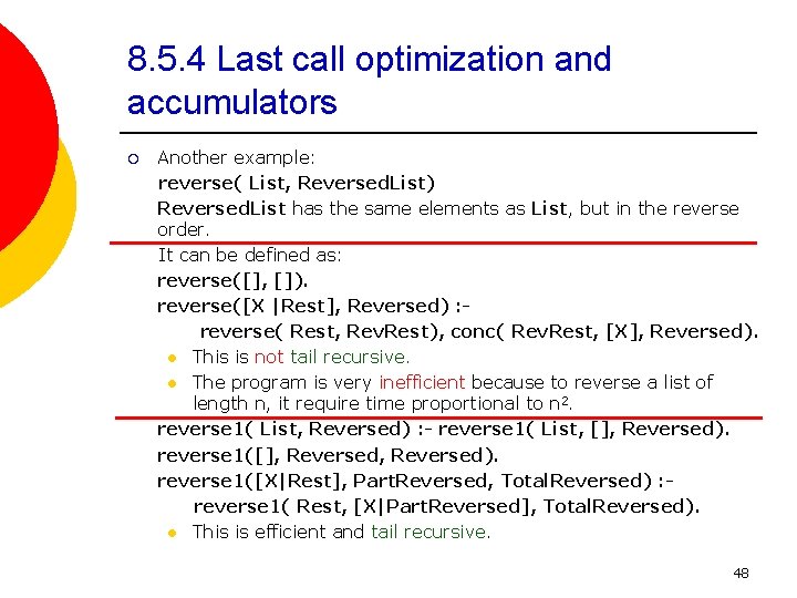
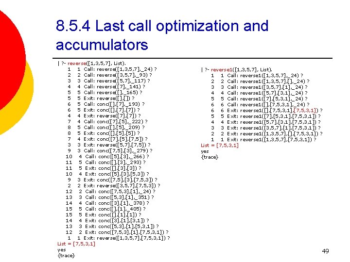
8. 5. 4 Last call optimization and accumulators ¡ Another example: reverse( List, Reversed. List) Reversed. List has the same elements as List, but in the reverse order. It can be defined as: reverse([], []). reverse([X |Rest], Reversed) : reverse( Rest, Rev. Rest), conc( Rev. Rest, [X], Reversed). l This is not tail recursive. l The program is very inefficient because to reverse a list of length n, it require time proportional to n 2. reverse 1( List, Reversed) : - reverse 1( List, [], Reversed). reverse 1([], Reversed). reverse 1([X|Rest], Part. Reversed, Total. Reversed) : reverse 1( Rest, [X|Part. Reversed], Total. Reversed). l This is efficient and tail recursive. 48

8. 5. 4 Last call optimization and accumulators | ? - reverse([1, 3, 5, 7], List). 1 1 Call: reverse([1, 3, 5, 7], _24) ? 2 2 Call: reverse([3, 5, 7], _93) ? 3 3 Call: reverse([5, 7], _117) ? 4 4 Call: reverse([7], _141) ? 5 5 Call: reverse([], _165) ? 5 5 Exit: reverse([], []) ? 6 5 Call: conc([], [7], _193) ? 6 5 Exit: conc([], [7]) ? 4 4 Exit: reverse([7], [7]) ? 7 4 Call: conc([7], [5], _222) ? 8 5 Call: conc([], [5], _209) ? 8 5 Exit: conc([], [5]) ? 7 4 Exit: conc([7], [5], [7, 5]) ? 3 3 Exit: reverse([5, 7], [7, 5]) ? 9 3 Call: conc([7, 5], [3], _279) ? 10 4 Call: conc([5], [3], _266) ? 11 5 Call: conc([], [3], _293) ? 11 5 Exit: conc([], [3]) ? 10 4 Exit: conc([5], [3], [5, 3]) ? 9 3 Exit: conc([7, 5], [3], [7, 5, 3]) ? 2 2 Exit: reverse([3, 5, 7], [7, 5, 3]) ? 12 2 Call: conc([7, 5, 3], [1], _24) ? 13 3 Call: conc([5, 3], [1], _351) ? 14 4 Call: conc([3], [1], _378) ? 15 5 Call: conc([], [1], _405) ? 15 5 Exit: conc([], [1]) ? 14 4 Exit: conc([3], [1], [3, 1]) ? 13 3 Exit: conc([5, 3], [1], [5, 3, 1]) ? 12 2 Exit: conc([7, 5, 3], [1], [7, 5, 3, 1]) ? 1 1 Exit: reverse([1, 3, 5, 7], [7, 5, 3, 1]) ? List = [7, 5, 3, 1] yes {trace} | ? - reverse 1([1, 3, 5, 7], List). 1 1 Call: reverse 1([1, 3, 5, 7], _24) ? 2 2 Call: reverse 1([1, 3, 5, 7], [], _24) ? 3 3 Call: reverse 1([3, 5, 7], [1], _24) ? 4 4 Call: reverse 1([5, 7], [3, 1], _24) ? 5 5 Call: reverse 1([7], [5, 3, 1], _24) ? 6 6 Call: reverse 1([], [7, 5, 3, 1], _24) ? 6 6 Exit: reverse 1([], [7, 5, 3, 1]) ? 5 5 Exit: reverse 1([7], [5, 3, 1], [7, 5, 3, 1]) ? 4 4 Exit: reverse 1([5, 7], [3, 1], [7, 5, 3, 1]) ? 3 3 Exit: reverse 1([3, 5, 7], [1], [7, 5, 3, 1]) ? 2 2 Exit: reverse 1([1, 3, 5, 7], [7, 5, 3, 1]) ? 1 1 Exit: reverse 1([1, 3, 5, 7], [7, 5, 3, 1]) ? List = [7, 5, 3, 1] yes {trace} 49

8. 5. 5 Simulating arrays with arg ¡ ¡ ¡ The list structure is the easiest representation for sets in Prolog. However, accessing an item in a list is done by scanning the list. For long lists this is very inefficient. In such cases, array structures are the most effective because they enable direct access to a required element. There is no array facility in Prolog, but array can be simulated to some extent by using the built-in predicates arg and functor. 50

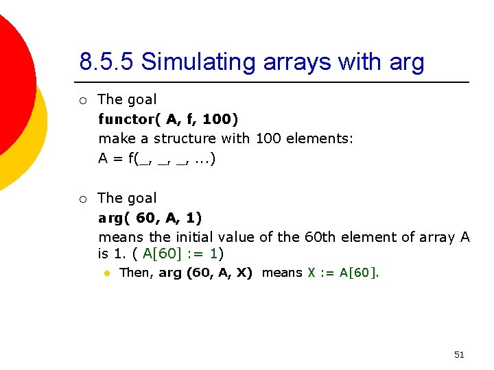
8. 5. 5 Simulating arrays with arg ¡ The goal functor( A, f, 100) make a structure with 100 elements: A = f(_, _, _, . . . ) ¡ The goal arg( 60, A, 1) means the initial value of the 60 th element of array A is 1. ( A[60] : = 1) l Then, arg (60, A, X) means X : = A[60]. 51

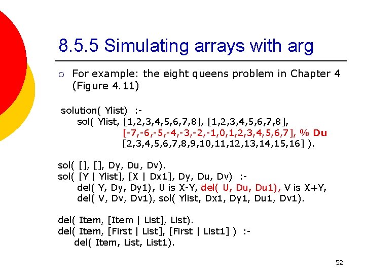
8. 5. 5 Simulating arrays with arg ¡ For example: the eight queens problem in Chapter 4 (Figure 4. 11) solution( Ylist) : sol( Ylist, [1, 2, 3, 4, 5, 6, 7, 8], [-7, -6, -5, -4, -3, -2, -1, 0, 1, 2, 3, 4, 5, 6, 7], % Du [2, 3, 4, 5, 6, 7, 8, 9, 10, 11, 12, 13, 14, 15, 16] ). sol( [], Dy, Du, Dv). sol( [Y | Ylist], [X | Dx 1], Dy, Du, Dv) : del( Y, Dy 1), U is X-Y, del( U, Du 1), V is X+Y, del( V, Dv 1), sol( Ylist, Dx 1, Dy 1, Du 1, Dv 1). del( Item, [Item | List], List). del( Item, [First | List], [First | List 1] ) : del( Item, List 1). 52

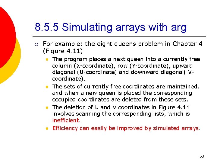
8. 5. 5 Simulating arrays with arg ¡ For example: the eight queens problem in Chapter 4 (Figure 4. 11) l l The program places a next queen into a currently free column (X-coordinate), row (Y-coordinate), upward diagonal (U-coordinate) and downward diagonal( Vcoordinate). The sets of currently free coordinates are maintained, and when a new queen is placed the corresponding occupied coordinates are deleted from these sets. The deletion of U and V coordinates in Figure 4. 11 involves scanning the corresponding lists, which is inefficient. Efficiency can easily be improved by simulated arrays. 53

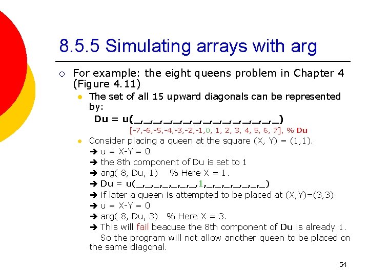
8. 5. 5 Simulating arrays with arg ¡ For example: the eight queens problem in Chapter 4 (Figure 4. 11) l The set of all 15 upward diagonals can be represented by: Du = u(_, _, _, _, _) [-7, -6, -5, -4, -3, -2, -1, 0, 1, 2, 3, 4, 5, 6, 7], % Du l Consider placing a queen at the square (X, Y) = (1, 1). u = X-Y = 0 the 8 th component of Du is set to 1 arg( 8, Du, 1) % Here X = 1. Du = u(_, _, 1, _, _, _, _) if later a queen is attempted to be placed at (X, Y)=(3, 3) u = X-Y = 0 arg( 8, Du, 3) % Here X = 3. This will fail beacuse the 8 th component of Du is already 1. So the program will not allow another queen to be placed on the same diagonal. 54

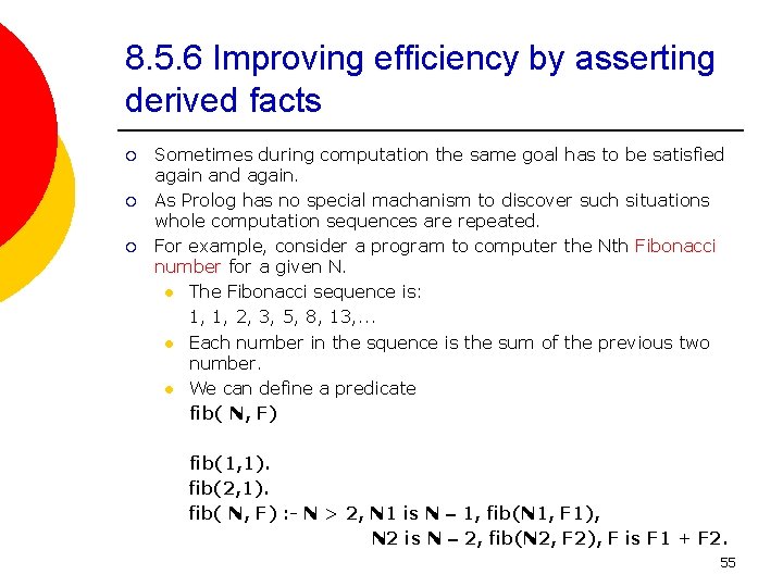
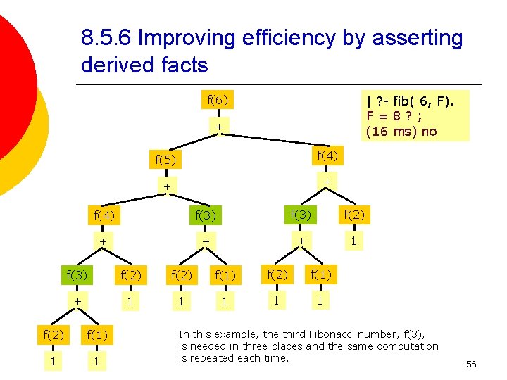
8. 5. 6 Improving efficiency by asserting derived facts ¡ ¡ ¡ Sometimes during computation the same goal has to be satisfied again and again. As Prolog has no special machanism to discover such situations whole computation sequences are repeated. For example, consider a program to computer the Nth Fibonacci number for a given N. l The Fibonacci sequence is: 1, 1, 2, 3, 5, 8, 13, . . . l Each number in the squence is the sum of the previous two number. l We can define a predicate fib( N, F) fib(1, 1). fib(2, 1). fib( N, F) : - N > 2, N 1 is N – 1, fib(N 1, F 1), N 2 is N – 2, fib(N 2, F 2), F is F 1 + F 2. 55

8. 5. 6 Improving efficiency by asserting derived facts | ? - fib( 6, F). F=8? ; (16 ms) no f(6) + f(5) f(4) + + f(4) f(3) f(2) + + + 1 f(3) f(2) f(1) + 1 1 1 f(2) f(1) 1 1 In this example, the third Fibonacci number, f(3), is needed in three places and the same computation is repeated each time. 56

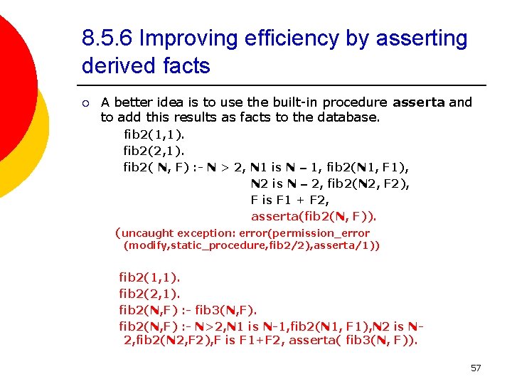
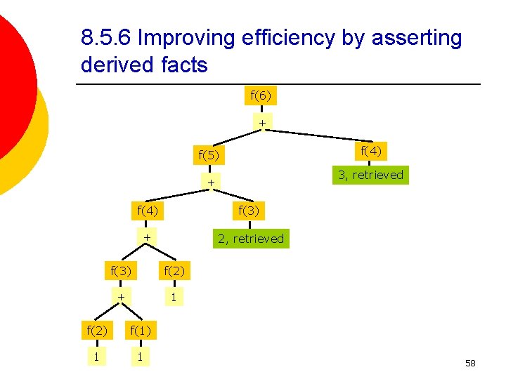
8. 5. 6 Improving efficiency by asserting derived facts ¡ A better idea is to use the built-in procedure asserta and to add this results as facts to the database. fib 2(1, 1). fib 2(2, 1). fib 2( N, F) : - N > 2, N 1 is N – 1, fib 2(N 1, F 1), N 2 is N – 2, fib 2(N 2, F 2), F is F 1 + F 2, asserta(fib 2(N, F)). (uncaught exception: error(permission_error (modify, static_procedure, fib 2/2), asserta/1)) fib 2(1, 1). fib 2(2, 1). fib 2(N, F) : - fib 3(N, F). fib 2(N, F) : - N>2, N 1 is N-1, fib 2(N 1, F 1), N 2 is N 2, fib 2(N 2, F 2), F is F 1+F 2, asserta( fib 3(N, F)). 57

8. 5. 6 Improving efficiency by asserting derived facts f(6) + f(4) f(5) 3, retrieved + f(4) f(3) + 2, retrieved f(3) f(2) + 1 f(2) f(1) 1 1 58

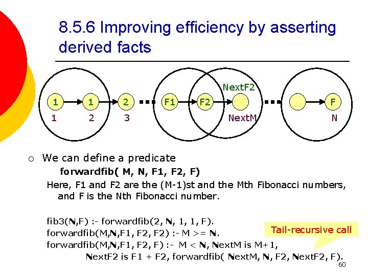
8. 5. 6 Improving efficiency by asserting derived facts ¡ ¡ ¡ Asserting intermediate results, also called caching(是一種將先前讀進 來的資料留著, 預備下一次讀取的技術), is a standard technique for avoiding repeated computations. It should be noted that we can preferably avoid repeated computation by using another algorithm, rather than by asserting intermediate results. The other algorithm will lead to a program that is more diffcult to understand, but more efficient to execute. The idea is not to define the Nth Fibonacci number simply as the sum of its two predecessors and leave the recursive calls to unfold( 展開) the whole computation ‘downwards’ to the two initial Fibonacci numbers. Instead, we can work ‘upwards’ starting with the initial two numbers, and compute the numbers in the sequence one by one in the forward direction. We have to stop when we have computed the Nth number. 59

8. 5. 6 Improving efficiency by asserting derived facts Next. F 2 ¡ 1 1 2 3 F 1 F 2 F Next. M N We can define a predicate forwardfib( M, N, F 1, F 2, F) Here, F 1 and F 2 are the (M-1)st and the Mth Fibonacci numbers, and F is the Nth Fibonacci number. fib 3(N, F) : - forwardfib(2, N, 1, 1, F). Tail-recursive call forwardfib(M, N, F 1, F 2) : - M >= N. forwardfib(M, N, F 1, F 2, F) : - M < N, Next. M is M+1, Next. F 2 is F 1 + F 2, forwardfib( Next. M, N, F 2, Next. F 2, F). 60

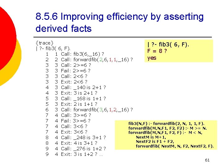
8. 5. 6 Improving efficiency by asserting derived facts {trace} | ? - fib 3( 6, F). F=8? 1 1 Call: fib 3(6, _16) ? yes 2 2 Call: forwardfib(2, 6, 1, 1, _16) ? 3 3 Call: 2>=6 ? 3 3 Fail: 2>=6 ? 3 3 Call: 2<6 ? 3 3 Exit: 2<6 ? 4 3 Call: _140 is 2+1 ? 4 3 Exit: 3 is 2+1 ? 5 3 Call: _168 is 1+1 ? 5 3 Exit: 2 is 1+1 ? 6 3 Call: forwardfib(3, 6, 1, 2, _16) ? 7 4 Call: 3>=6 ? 7 4 Fail: 3>=6 ? fib 3(N, F) : - forwardfib(2, N, 1, 1, F). 7 4 Call: 3<6 ? forwardfib(M, N, F 1, F 2) : - M >= N. 7 4 Exit: 3<6 ? forwardfib(M, N, F 1, F 2, F) : - M < N, Next. M is M+1, 8 4 Call: _248 is 3+1 ? Next. F 2 is F 1 + F 2, 8 4 Exit: 4 is 3+1 ? forwardfib( Next. M, N, F 2, Next. F 2, F). 9 4 Call: _276 is 1+2 ? 9 4 Exit: 3 is 1+2 ? … 61

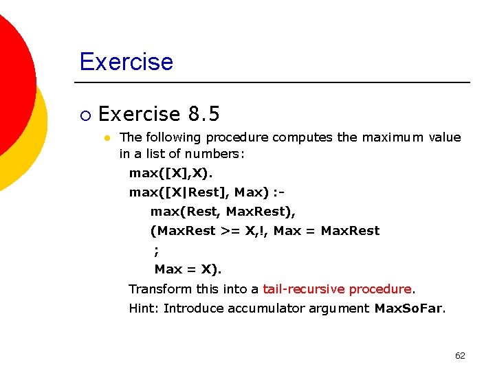
Exercise ¡ Exercise 8. 5 l The following procedure computes the maximum value in a list of numbers: max([X], X). max([X|Rest], Max) : max(Rest, Max. Rest), (Max. Rest >= X, !, Max = Max. Rest ; Max = X). Transform this into a tail-recursive procedure. Hint: Introduce accumulator argument Max. So. Far. 62