Part 1 Review Science depends on repeatable data

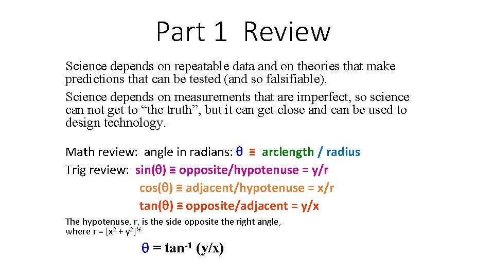
Part 1 Review Science depends on repeatable data and on theories that make predictions that can be tested (and so falsifiable). Science depends on measurements that are imperfect, so science can not get to “the truth”, but it can get close and can be used to design technology. Math review: angle in radians: ≡ arclength / radius Trig review: sin( ) ≡ opposite/hypotenuse = y/r cos( ) ≡ adjacent/hypotenuse = x/r tan( ) ≡ opposite/adjacent = y/x The hypotenuse, r, is the side opposite the right angle, where r = [x 2 + y 2]½ = tan-1 (y/x)

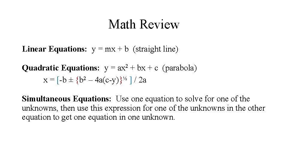
Math Review Linear Equations: y = mx + b (straight line) Quadratic Equations: y = ax 2 + bx + c (parabola) x = [-b ± {b 2 – 4 a(c-y)}½ ] / 2 a Simultaneous Equations: Use one equation to solve for one of the unknowns, then use this expression for one of the unknowns in the other equation to get one equation in one unknown.

Metric System basics: (MKS system) length (in Meters) amount of “stuff” called mass (in Kilograms) time (in Seconds) Prefixes centimeter (cm) =. 01 meters = 10 -2 m millimeter (mm) =. 001 meters = 10 -3 m micrometer ( m) =. 000001 meters = 10 -6 m nanometer (nm) =. 00001 meters = 10 -9 m picometer (pm) =. 0000001 meters = 10 -12 m kilo (km) = 1, 000 meters = 103 m mega (Mm) = 1, 000 meters = 106 m giga (Gm) = 1, 000, 000 meters = 109 m tera (Tm) = 1, 000, 000 meters = 1012 m

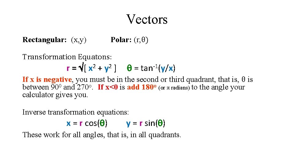
Vectors Rectangular: (x, y) Polar: (r, θ) Transformation Equatons: r = [ x 2 + y 2 ] = tan-1(y/x) If x is negative, you must be in the second or third quadrant, that is, θ is between 900 and 270 o. If x<0 is add 180 o (or π radians) to the angle your calculator gives you. Inverse transformation equations: x = r cos( ) y = r sin( ) These work for all angles, that is, in all quadrants.

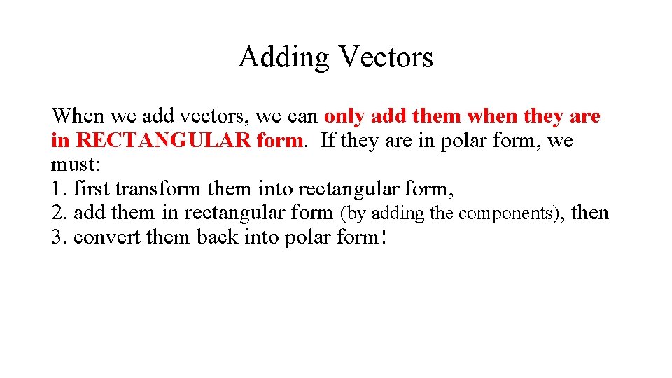
Adding Vectors When we add vectors, we can only add them when they are in RECTANGULAR form. If they are in polar form, we must: 1. first transform them into rectangular form, 2. add them in rectangular form (by adding the components), then 3. convert them back into polar form!

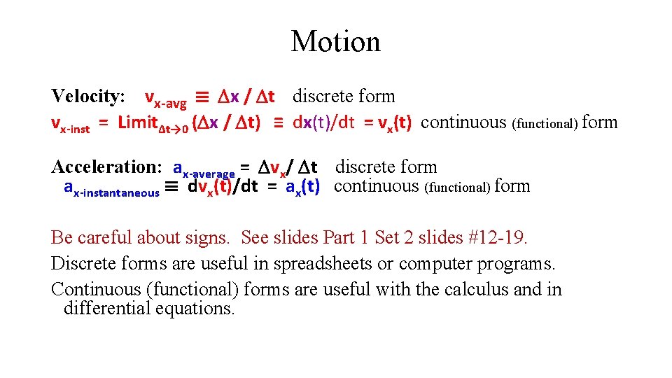
Motion Velocity: vx-avg ≡ x / t discrete form vx-inst = LimitΔt→ 0 ( x / t) ≡ dx(t)/dt = vx(t) continuous (functional) form Acceleration: ax-average = vx/ t discrete form ax-instantaneous ≡ dvx(t)/dt = ax(t) continuous (functional) form Be careful about signs. See slides Part 1 Set 2 slides #12 -19. Discrete forms are useful in spreadsheets or computer programs. Continuous (functional) forms are useful with the calculus and in differential equations.

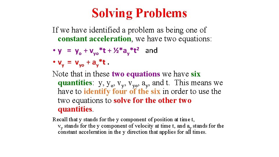
Solving Problems If we have identified a problem as being one of constant acceleration, we have two equations: • y = yo + vyo*t + ½*ay*t 2 and • vy = vyo + ay*t. Note that in these two equations we have six quantities: y, yo, vyo, ay, and t. This means we have to identify four of the six in order to use the two equations to solve for the other two quantities. Recall that y stands for the y component of position at time t, vy stands for the y component of velocity at time t, and ay stands for the constant acceleration in the y direction that applies for all times.

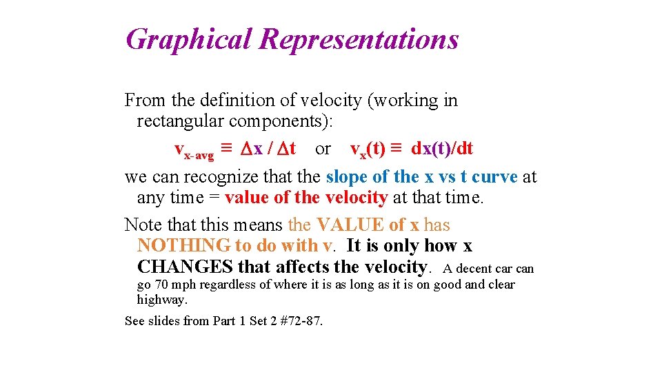
Graphical Representations From the definition of velocity (working in rectangular components): vx-avg ≡ x / t or vx(t) ≡ dx(t)/dt we can recognize that the slope of the x vs t curve at any time = value of the velocity at that time. Note that this means the VALUE of x has NOTHING to do with v. It is only how x CHANGES that affects the velocity. A decent car can go 70 mph regardless of where it is as long as it is on good and clear highway. See slides from Part 1 Set 2 #72 -87.