Part 1 Probability and Distribution Theory Statistical Inference
Part 1 – Probability and Distribution Theory Statistical Inference and Regression Analysis: Stat-GB. 3302. 30, Stat-UB. 0015. 01 Professor William Greene Stern School of Business IOMS Department of Economics
Part 1 – Probability and Distribution Theory Part 1 –Probability and Distribution Theory
Part 1 – Probability and Distribution Theory 1 – Probability
Part 1 – Probability and Distribution Theory 4/116 The Sample Space ¢ Collection of possible outcomes l l l ¢ Random outcomes: The result of a process l l l ¢ Exclusive Exhaustive Ω = {the set of possible outcomes} Sequence of events, Number of events, Measurement of a length of time, space, etc. Outcomes, experiments and sample spaces
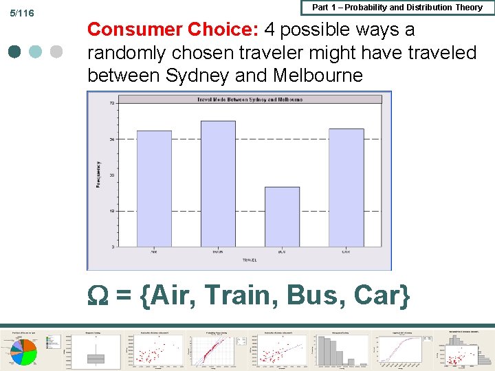
5/116 Part 1 – Probability and Distribution Theory Consumer Choice: 4 possible ways a randomly chosen traveler might have traveled between Sydney and Melbourne = {Air, Train, Bus, Car}
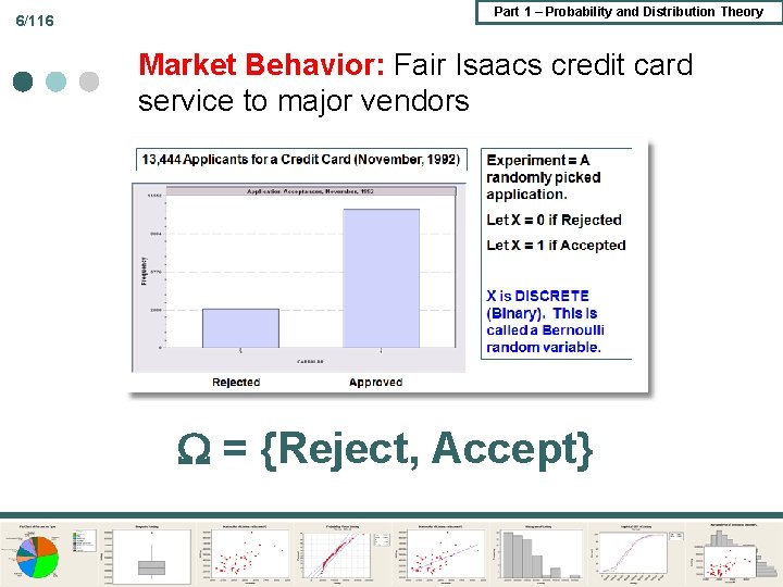
6/116 Part 1 – Probability and Distribution Theory Market Behavior: Fair Isaacs credit card service to major vendors = {Reject, Accept}
Part 1 – Probability and Distribution Theory 7/116 Measurement of Lifetimes ¢ A box of light bulbs states “Average life is 1500 hours” ¢ Outcome = length of time until failure (lifetime) of a randomly chosen light bulb = {lifetime | lifetime > 0}
Part 1 – Probability and Distribution Theory 8/116 Events ¢ ¢ Events are defined as l Subsets of sample space, such as empty set l Intersection of related events l Complements such as “A” and “not A” l Disjoint sets such as (train, bus), (air, car) Any subset including is a disjoint union of subsets: = (Air, Train) (Bus, Car)
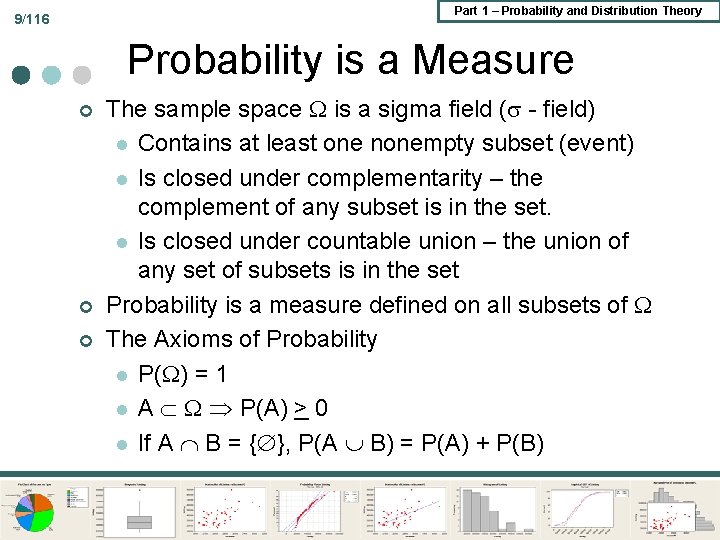
Part 1 – Probability and Distribution Theory 9/116 Probability is a Measure ¢ ¢ ¢ The sample space is a sigma field ( - field) l Contains at least one nonempty subset (event) l Is closed under complementarity – the complement of any subset is in the set. l Is closed under countable union – the union of any set of subsets is in the set Probability is a measure defined on all subsets of The Axioms of Probability l P( ) = 1 l A P(A) > 0 l If A B = { }, P(A B) = P(A) + P(B)
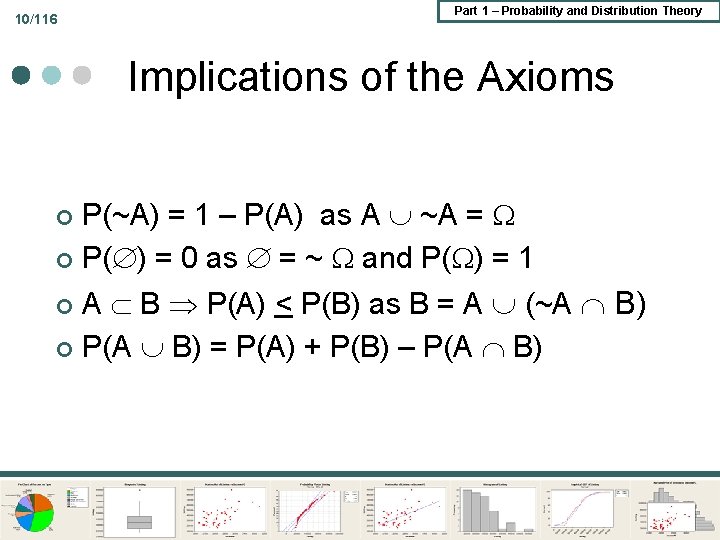
10/116 Part 1 – Probability and Distribution Theory Implications of the Axioms P(~A) = 1 – P(A) as A ~A = ¢ P( ) = 0 as = ~ and P( ) = 1 ¢ A B P(A) < P(B) as B = A (~A B) ¢ P(A B) = P(A) + P(B) – P(A B) ¢
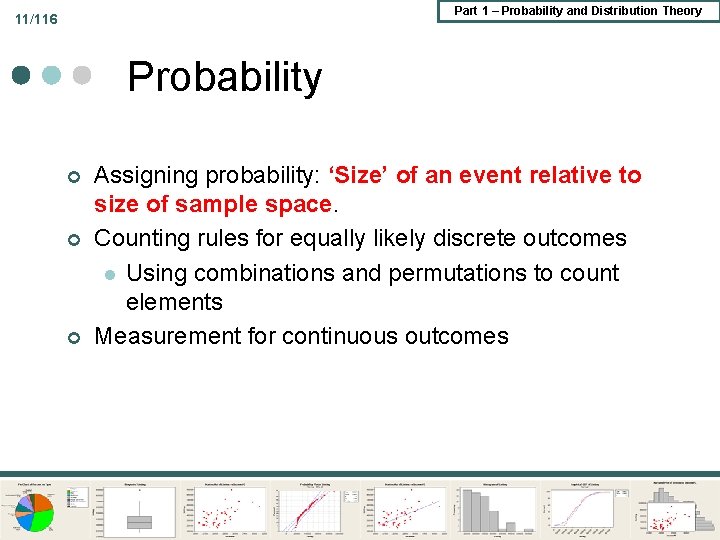
Part 1 – Probability and Distribution Theory 11/116 Probability ¢ ¢ ¢ Assigning probability: ‘Size’ of an event relative to size of sample space. Counting rules for equally likely discrete outcomes l Using combinations and permutations to count elements Measurement for continuous outcomes
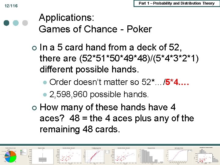
Part 1 – Probability and Distribution Theory 12/116 Applications: Games of Chance - Poker ¢ In a 5 card hand from a deck of 52, there are (52*51*50*49*48)/(5*4*3*2*1) different possible hands. Order doesn’t matter so 52*…/5*4…. l 2, 598, 960 possible hands. l ¢ How many of these hands have 4 aces? 48 = the 4 aces plus any of the remaining 48 cards.
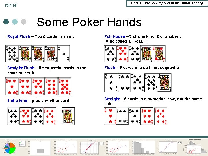
Part 1 – Probability and Distribution Theory 13/116 Some Poker Hands Royal Flush – Top 5 cards in a suit Full House – 3 of one kind, 2 of another. (Also called a “boat. ”) Straight Flush – 5 sequential cards in the same suit Flush – 5 cards in a suit, not sequential 4 of a kind – plus any other card Straight – 5 cards in a numerical row, not the same suit
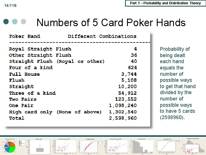
14/116 Part 1 – Probability and Distribution Theory Numbers of 5 Card Poker Hands Probability of being dealt each hand equals the number of possible ways to get that hand divided by the number of possible ways to have 5 cards (2598960).
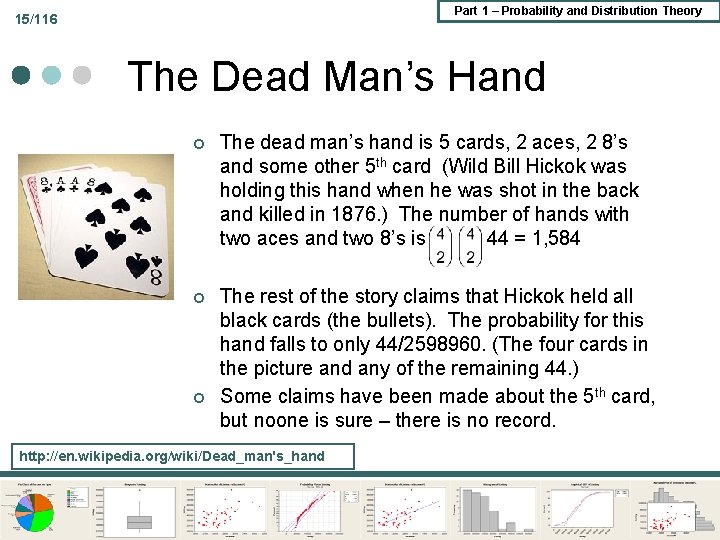
Part 1 – Probability and Distribution Theory 15/116 The Dead Man’s Hand ¢ The dead man’s hand is 5 cards, 2 aces, 2 8’s and some other 5 th card (Wild Bill Hickok was holding this hand when he was shot in the back and killed in 1876. ) The number of hands with two aces and two 8’s is 44 = 1, 584 ¢ The rest of the story claims that Hickok held all black cards (the bullets). The probability for this hand falls to only 44/2598960. (The four cards in the picture and any of the remaining 44. ) Some claims have been made about the 5 th card, but noone is sure – there is no record. ¢ http: //en. wikipedia. org/wiki/Dead_man's_hand
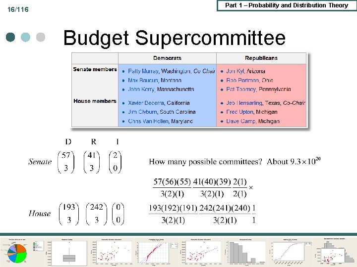
16/116 Part 1 – Probability and Distribution Theory Budget Supercommittee
17/116 Part 1 – Probability and Distribution Theory Conditional Probability ¢ ¢ Probability of event A given that event B occurs. P(A|B) = P(A, B)/P(B) = Size of A relative to a subset of Basic result p(A, B) = p(A|B) p(B) (follows from the definition) Useful application: Bayes theorem l Applications – mammography, drug testing, lie detector test, PSA test.
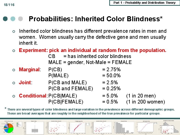
18/116 Part 1 – Probability and Distribution Theory Probabilities: Inherited Color Blindness* ¢ ¢ ¢ Inherited color blindness has different prevalence rates in men and women. Women usually carry the defective gene and men usually inherit it. Experiment: pick an individual at random from the population. CB = has inherited color blindness MALE = gender, Not-Male = FEMALE Marginal: P(CB) = 2. 75% P(MALE) = 50. 0% Joint: P(CB and MALE) = 2. 5% P(CB and FEMALE) = 0. 25% Conditional: P(CB|MALE) = 5. 0% (1 in 20 men) P(CB|FEMALE) = 0. 5% (1 in 200 women) * There are several types of color blindness and large variation in the prevalence across different demographic groups. These are broad averages that are roughly in the neighborhood of the true prevalence for particular groups.
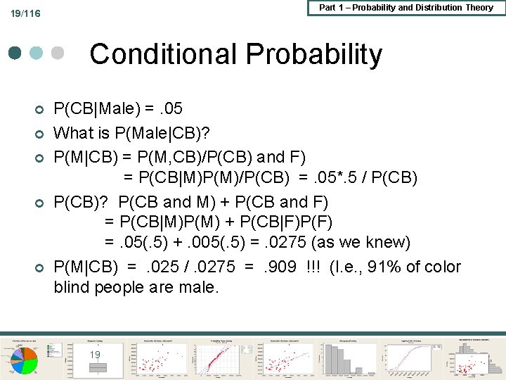
Part 1 – Probability and Distribution Theory 19/116 Conditional Probability ¢ ¢ ¢ P(CB|Male) =. 05 What is P(Male|CB)? P(M|CB) = P(M, CB)/P(CB) and F) = P(CB|M)P(M)/P(CB) =. 05*. 5 / P(CB)? P(CB and M) + P(CB and F) = P(CB|M)P(M) + P(CB|F)P(F) =. 05(. 5) +. 005(. 5) =. 0275 (as we knew) P(M|CB) =. 025 /. 0275 =. 909 !!! (I. e. , 91% of color blind people are male. 19
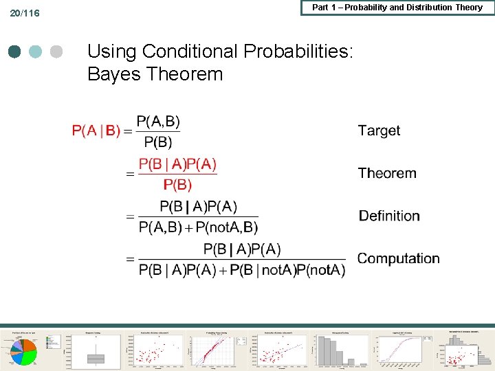
20/116 Part 1 – Probability and Distribution Theory Using Conditional Probabilities: Bayes Theorem
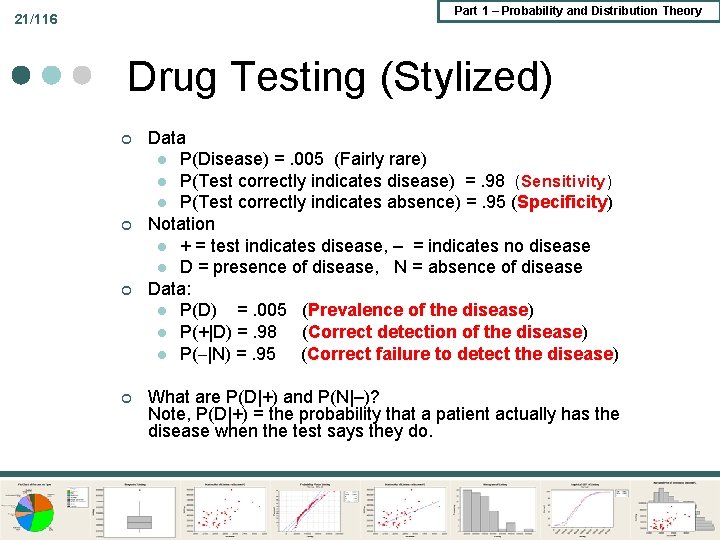
Part 1 – Probability and Distribution Theory 21/116 Drug Testing (Stylized) ¢ ¢ Data l P(Disease) =. 005 (Fairly rare) l P(Test correctly indicates disease) =. 98 (Sensitivity) l P(Test correctly indicates absence) =. 95 (Specificity) Notation l + = test indicates disease, – = indicates no disease l D = presence of disease, N = absence of disease Data: l P(D) =. 005 (Prevalence of the disease) l P(+|D) =. 98 (Correct detection of the disease) l P(–|N) =. 95 (Correct failure to detect the disease) What are P(D|+) and P(N|–)? Note, P(D|+) = the probability that a patient actually has the disease when the test says they do.
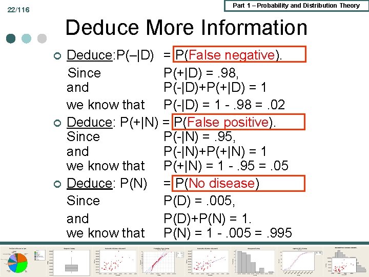
Part 1 – Probability and Distribution Theory 22/116 Deduce More Information ¢ ¢ ¢ Deduce: P(–|D) = P(False negative). Since P(+|D) =. 98, and P(-|D)+P(+|D) = 1 we know that P(-|D) = 1 -. 98 =. 02 Deduce: P(+|N) = P(False positive). Since P(-|N) =. 95, and P(-|N)+P(+|N) = 1 we know that P(+|N) = 1 -. 95 =. 05 Deduce: P(N) = P(No disease) Since P(D) =. 005, and P(D)+P(N) = 1. we know that P(N) = 1 -. 005 =. 995
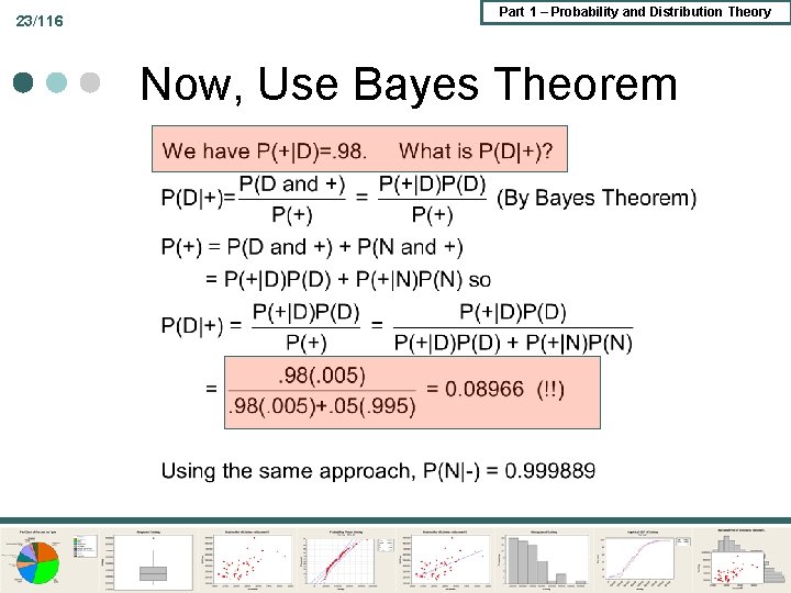
23/116 Part 1 – Probability and Distribution Theory Now, Use Bayes Theorem
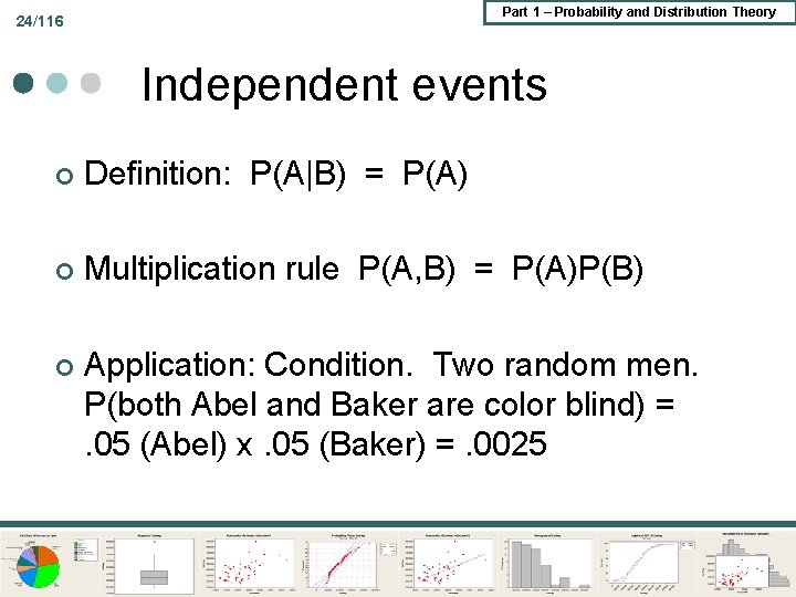
Part 1 – Probability and Distribution Theory 24/116 Independent events ¢ Definition: P(A|B) = P(A) ¢ Multiplication rule P(A, B) = P(A)P(B) ¢ Application: Condition. Two random men. P(both Abel and Baker are color blind) =. 05 (Abel) x. 05 (Baker) =. 0025
Part 1 – Probability and Distribution Theory 2 – Random Variables
Part 1 – Probability and Distribution Theory 26/116 Random Variable Definition: Maps elements of the sample space to a variable: ¢ Assigns a value to ¢ Types of random variables ¢ Discrete: Payoff to poker hands l Continuous: Lightbulb lifetimes l Mixed: Ticket sales with capacity constraints. (Censoring) l
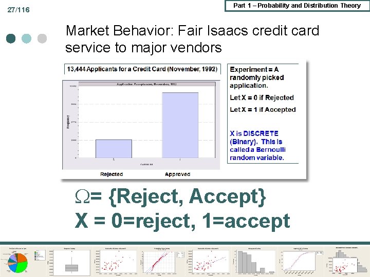
27/116 Part 1 – Probability and Distribution Theory Market Behavior: Fair Isaacs credit card service to major vendors = {Reject, Accept} X = 0=reject, 1=accept
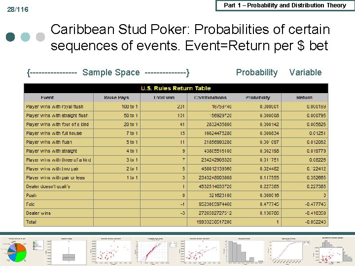
Part 1 – Probability and Distribution Theory 28/116 Caribbean Stud Poker: Probabilities of certain sequences of events. Event=Return per $ bet {-------- Sample Space -------} Probability Variable
Part 1 – Probability and Distribution Theory 29/116 Features of Random Variables ¢ Probability Distribution Mass function: Prob(X=x)=f(x) l Density function: f(x), x =. . . l ¢ Cumulative probabilities; CDF Prob(X < x) l F(x) l ¢ Quantiles: x such that F(x) = Q l Median: x = median, Q = 0. 5.
Part 1 – Probability and Distribution Theory 30/116 Discrete Random Variables ¢ ¢ ¢ Elemental building block l Bernoulli: Credit card applications l Discrete uniform: Die toss Counting Rules l Binomial: Family composition l Hypergeometric: House/Senate Supercommittee Models l Poisson: Diabetes prevalence, Accidents, etc.
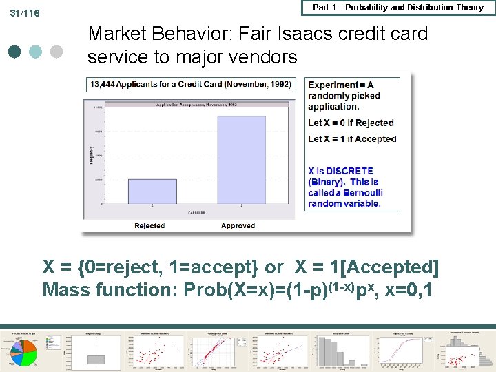
31/116 Part 1 – Probability and Distribution Theory Market Behavior: Fair Isaacs credit card service to major vendors X = {0=reject, 1=accept} or X = 1[Accepted] Mass function: Prob(X=x)=(1 -p)(1 -x)px, x=0, 1
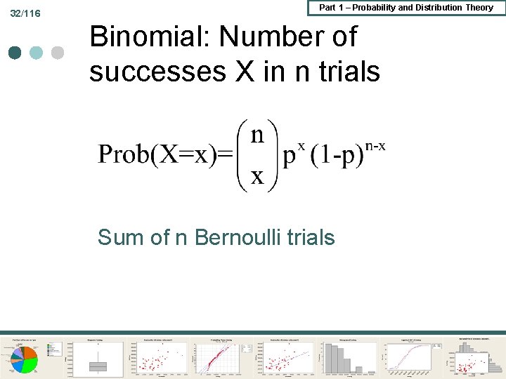
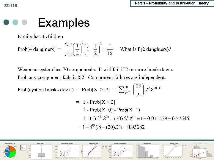
32/116 Part 1 – Probability and Distribution Theory Binomial: Number of successes X in n trials Sum of n Bernoulli trials
Part 1 – Probability and Distribution Theory 33/116 Examples
Part 1 – Probability and Distribution Theory 34/116 Poisson ¢ Approximation to binomial ¢ General model for a type of process
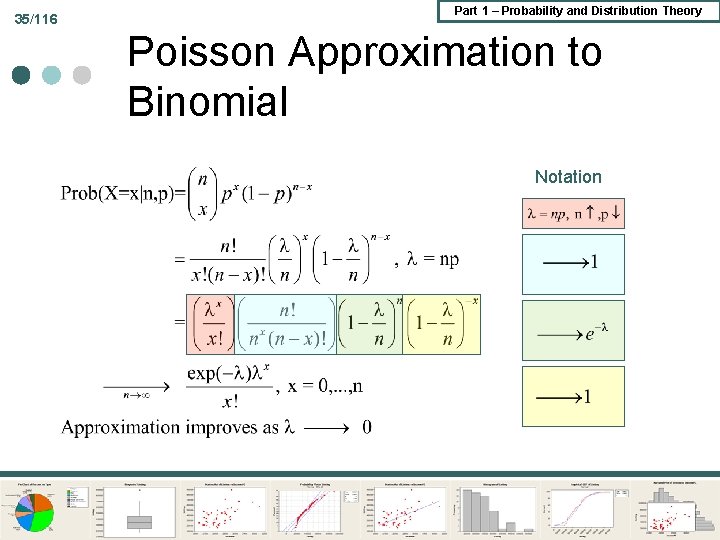
35/116 Part 1 – Probability and Distribution Theory Poisson Approximation to Binomial Notation
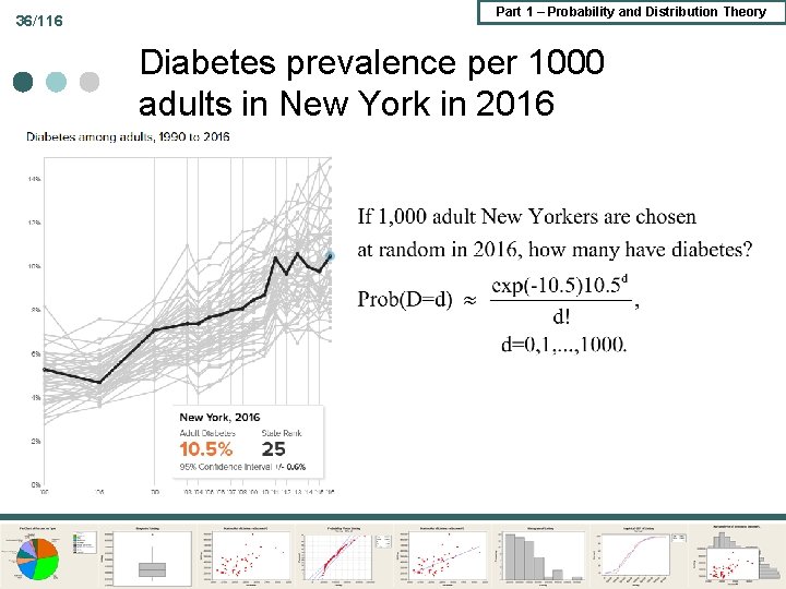
36/116 Part 1 – Probability and Distribution Theory Diabetes prevalence per 1000 adults in New York in 2016
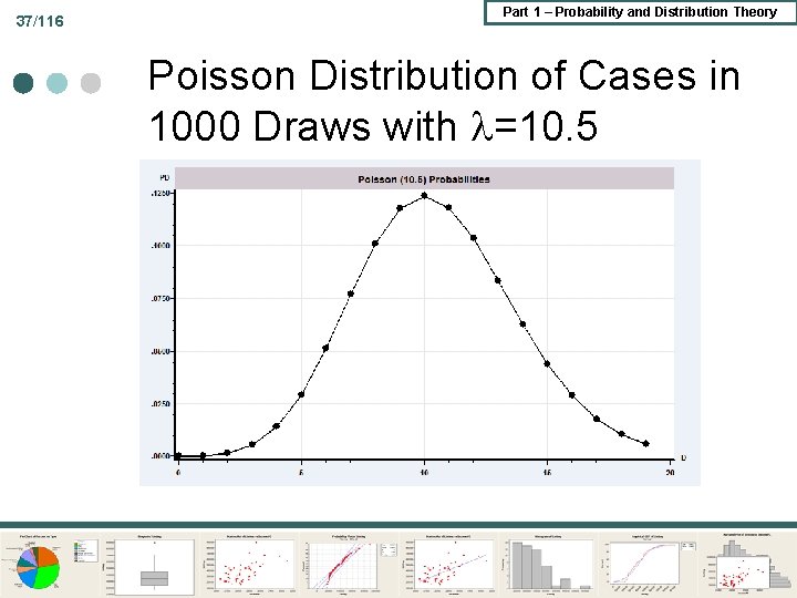
37/116 Part 1 – Probability and Distribution Theory Poisson Distribution of Cases in 1000 Draws with =10. 5
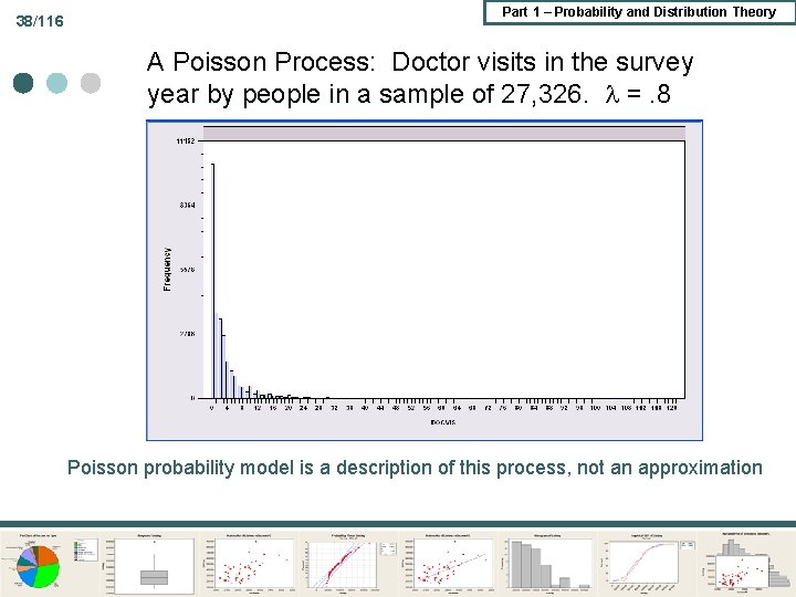
38/116 Part 1 – Probability and Distribution Theory A Poisson Process: Doctor visits in the survey year by people in a sample of 27, 326. =. 8 Poisson probability model is a description of this process, not an approximation
Part 1 – Probability and Distribution Theory 39/116 Continuous Random Variable Models of probabilities attached to events. ¢ Density function, f(x) ¢ Probability measure P(event) obtained using the density. ¢ Application: Lightbulb lifetimes ¢
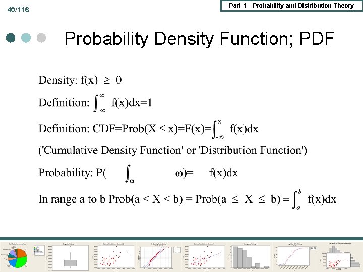
40/116 Part 1 – Probability and Distribution Theory Probability Density Function; PDF

41/116 Part 1 – Probability and Distribution Theory A Model for Light Bulb Lifetimes This is the exponential model for lifetimes. The model is f(time) = (1/μ) e-time/μ
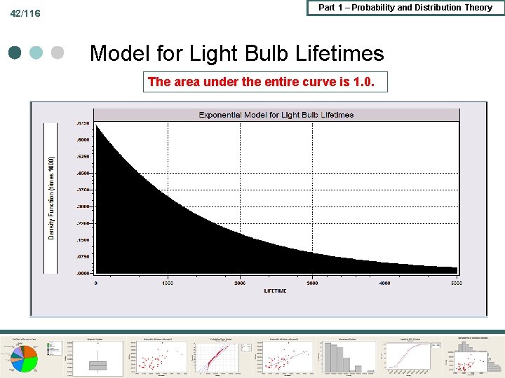
42/116 Part 1 – Probability and Distribution Theory Model for Light Bulb Lifetimes The area under the entire curve is 1. 0.
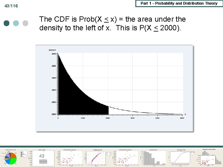
Part 1 – Probability and Distribution Theory 43/116 The CDF is Prob(X < x) = the area under the density to the left of x. This is P(X < 2000). 43
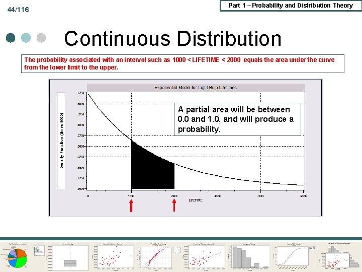
44/116 Part 1 – Probability and Distribution Theory Continuous Distribution The probability associated with an interval such as 1000 < LIFETIME < 2000 equals the area under the curve from the lower limit to the upper. A partial area will be between 0. 0 and 1. 0, and will produce a probability.
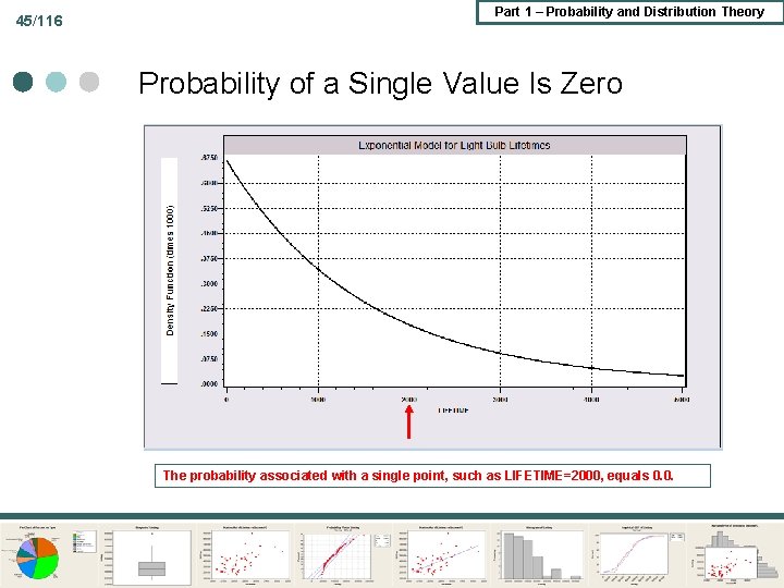
45/116 Part 1 – Probability and Distribution Theory Probability of a Single Value Is Zero The probability associated with a single point, such as LIFETIME=2000, equals 0. 0.
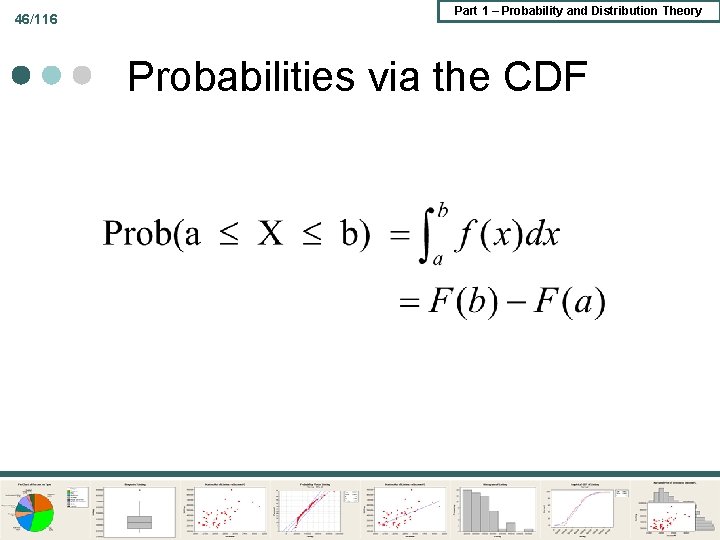
46/116 Part 1 – Probability and Distribution Theory Probabilities via the CDF
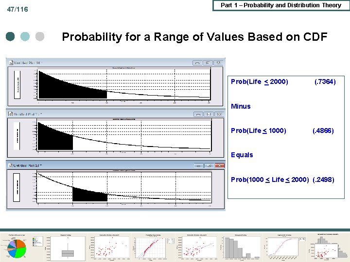
47/116 Part 1 – Probability and Distribution Theory Probability for a Range of Values Based on CDF Prob(Life < 2000) (. 7364) Minus Prob(Life < 1000) (. 4866) Equals Prob(1000 < Life < 2000) (. 2498)
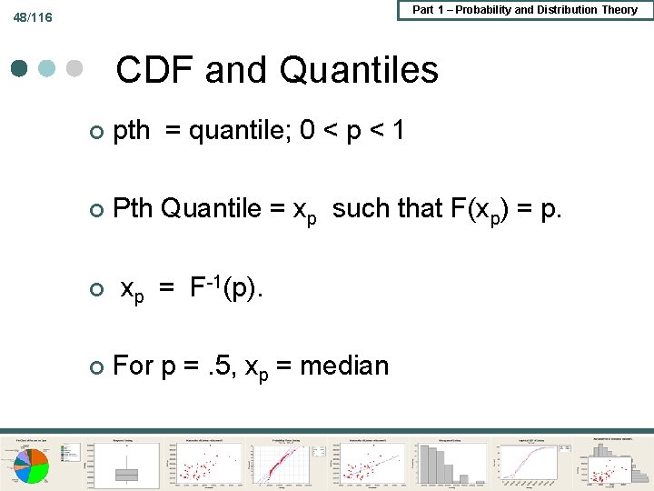
Part 1 – Probability and Distribution Theory 48/116 CDF and Quantiles ¢ pth = quantile; 0 < p < 1 ¢ Pth Quantile = xp such that F(xp) = p. ¢ ¢ xp = F-1(p). For p =. 5, xp = median
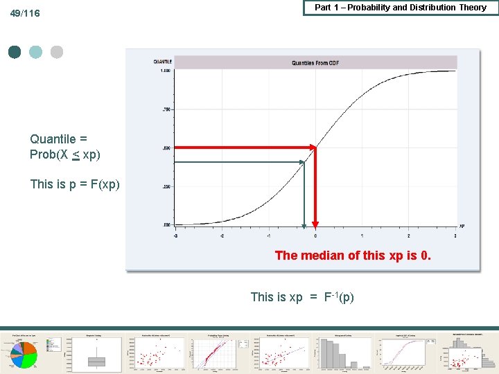
49/116 Part 1 – Probability and Distribution Theory Quantile = Prob(X < xp) This is p = F(xp) The median of this xp is 0. This is xp = F-1(p)
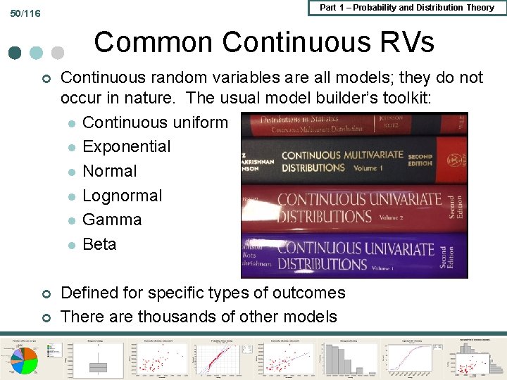
Part 1 – Probability and Distribution Theory 50/116 Common Continuous RVs ¢ Continuous random variables are all models; they do not occur in nature. The usual model builder’s toolkit: l Continuous uniform l Exponential l Normal l Lognormal l Gamma l Beta ¢ Defined for specific types of outcomes There are thousands of other models ¢
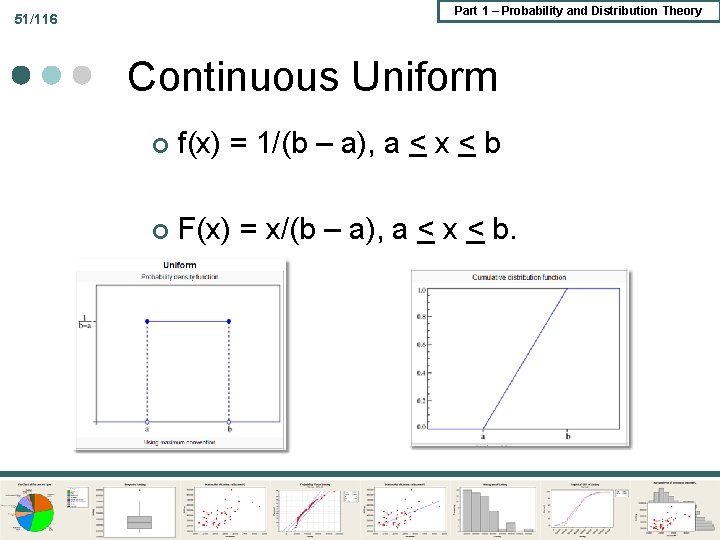
Part 1 – Probability and Distribution Theory 51/116 Continuous Uniform ¢ f(x) = 1/(b – a), a < x < b ¢ F(x) = x/(b – a), a < x < b.
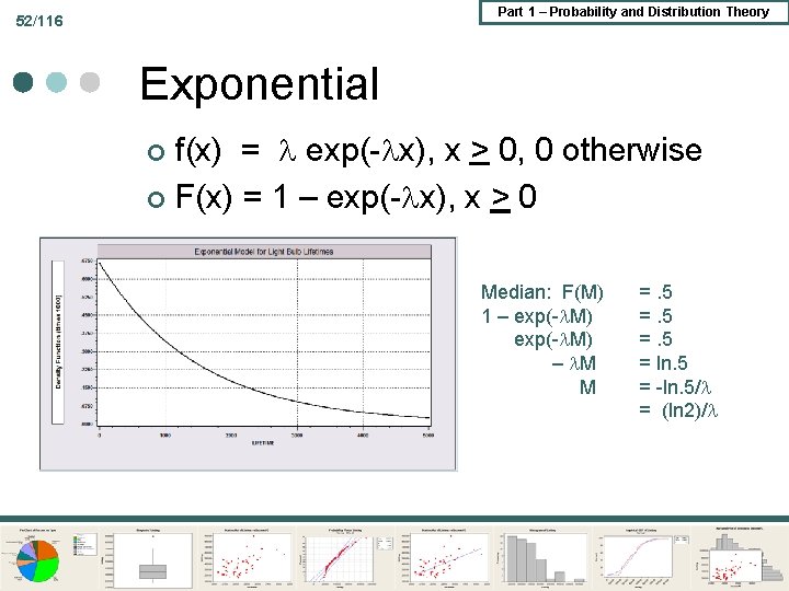
Part 1 – Probability and Distribution Theory 52/116 Exponential f(x) = exp(- x), x > 0, 0 otherwise ¢ F(x) = 1 – exp(- x), x > 0 ¢ Median: F(M) 1 – exp(- M) – M M =. 5 = ln. 5 = -ln. 5/ = (ln 2)/
Part 1 – Probability and Distribution Theory 53/116 53

54/116 Part 1 – Probability and Distribution Theory Gamma Density Uses the Gamma Function
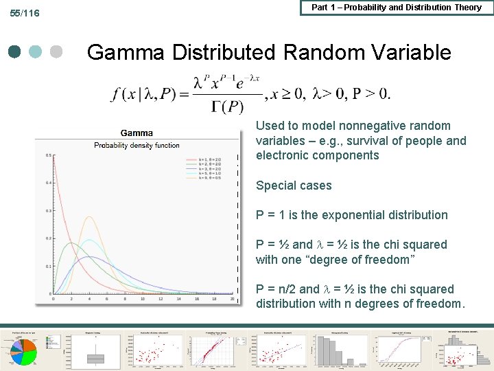
55/116 Part 1 – Probability and Distribution Theory Gamma Distributed Random Variable Used to model nonnegative random variables – e. g. , survival of people and electronic components Special cases P = 1 is the exponential distribution P = ½ and = ½ is the chi squared with one “degree of freedom” P = n/2 and = ½ is the chi squared distribution with n degrees of freedom.

56/116 Part 1 – Probability and Distribution Theory Beta Uses Beta Integrals

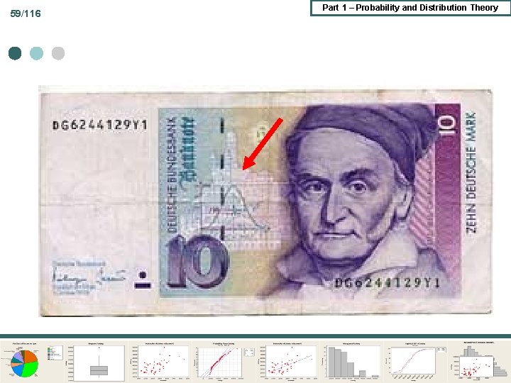
57/116 Part 1 – Probability and Distribution Theory Normal Density – THE Model Mean = μ, standard deviation = σ
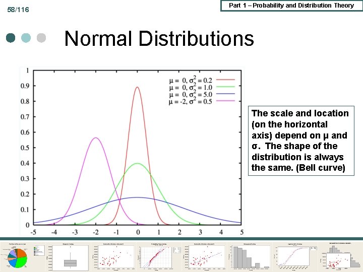
58/116 Part 1 – Probability and Distribution Theory Normal Distributions The scale and location (on the horizontal axis) depend on μ and σ. The shape of the distribution is always the same. (Bell curve)
59/116 Part 1 – Probability and Distribution Theory
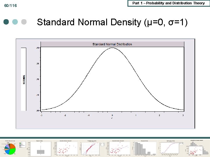
60/116 Part 1 – Probability and Distribution Theory Standard Normal Density (μ=0, σ=1)
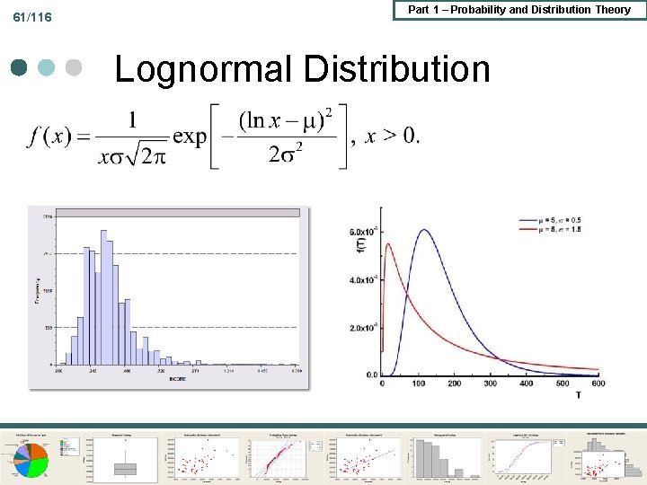
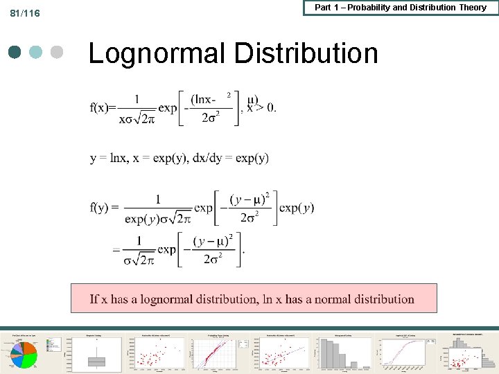
61/116 Part 1 – Probability and Distribution Theory Lognormal Distribution
Part 1 – Probability and Distribution Theory 62/116 Censoring and Truncation ¢ ¢ Censoring l Observation mechanism. Values above or below a certain value are assigned the boundary value l Applications, ticket market: demand vs. sales given capacity constraints; top coded income data Truncation l Observation mechanism. The relevant distribution only applies in a restricted range of the random variable l Application: On site survey for recreation visits. Truncated Poisson l Incidental truncation: Income is observed only for those wealth (not income) exceeds $100, 000.
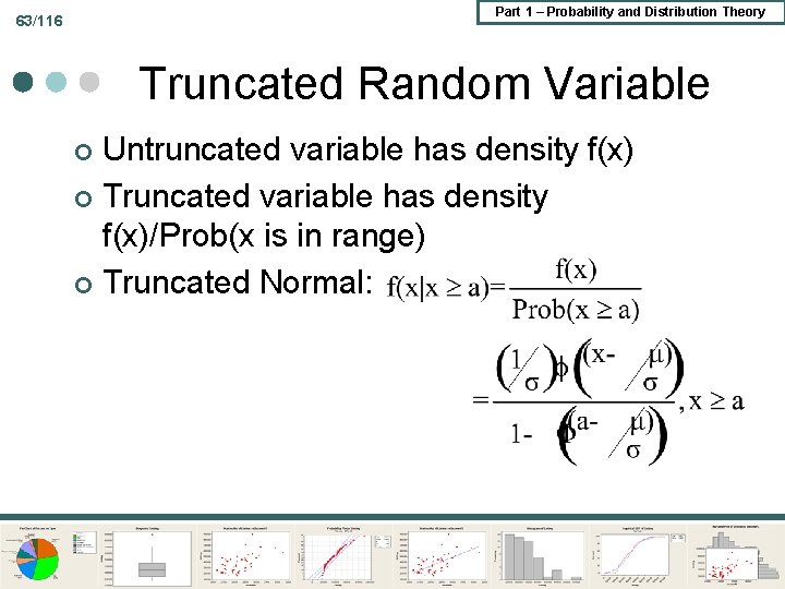
Part 1 – Probability and Distribution Theory 63/116 Truncated Random Variable Untruncated variable has density f(x) ¢ Truncated variable has density f(x)/Prob(x is in range) ¢ Truncated Normal: ¢
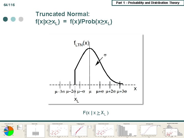
Part 1 – Probability and Distribution Theory 64/116 Truncated Normal: f(x|x>x. L) = f(x)/Prob(x>x. L) F(x | x > XL )
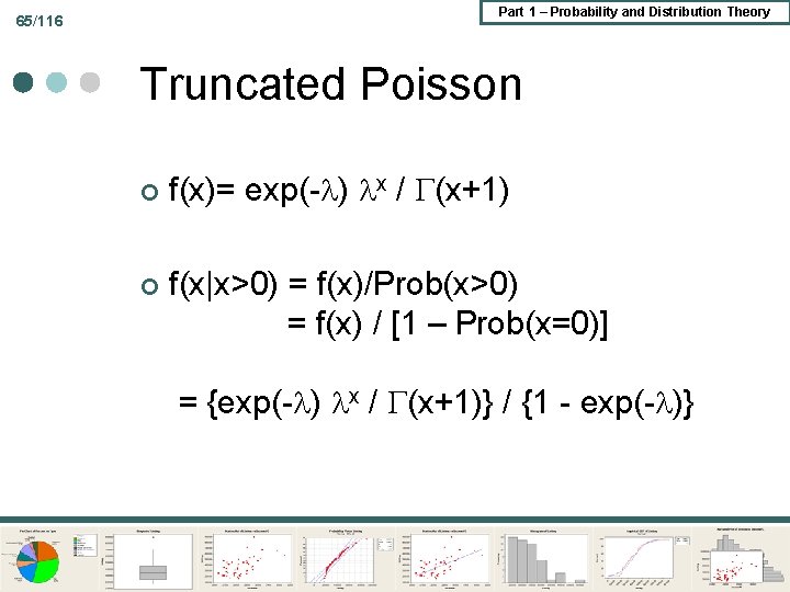
Part 1 – Probability and Distribution Theory 65/116 Truncated Poisson ¢ ¢ f(x)= exp(- ) x / (x+1) f(x|x>0) = f(x)/Prob(x>0) = f(x) / [1 – Prob(x=0)] = {exp(- ) x / (x+1)} / {1 - exp(- )}
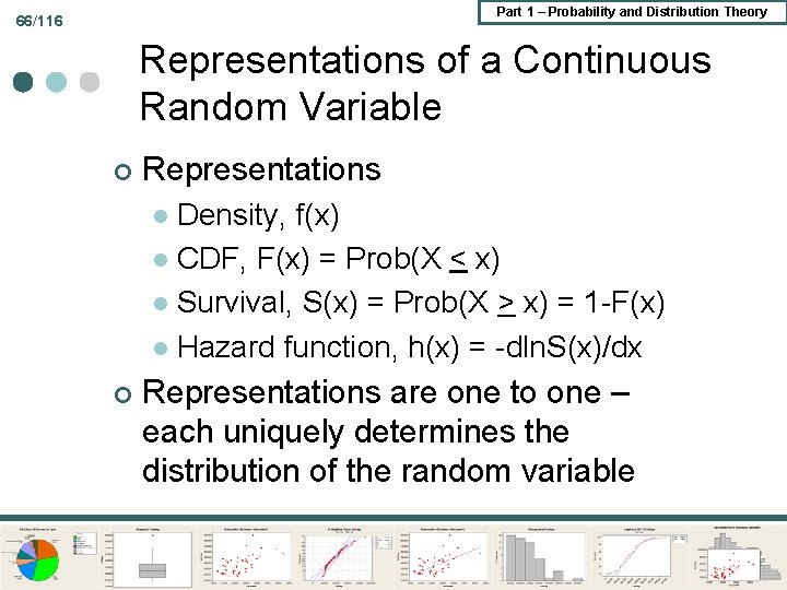
Part 1 – Probability and Distribution Theory 66/116 Representations of a Continuous Random Variable ¢ Representations Density, f(x) l CDF, F(x) = Prob(X < x) l Survival, S(x) = Prob(X > x) = 1 -F(x) l Hazard function, h(x) = -dln. S(x)/dx l ¢ Representations are one to one – each uniquely determines the distribution of the random variable
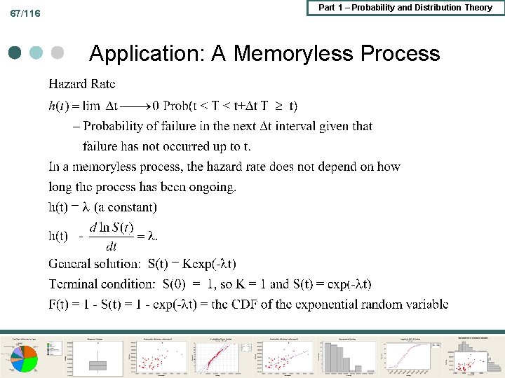
67/116 Part 1 – Probability and Distribution Theory Application: A Memoryless Process
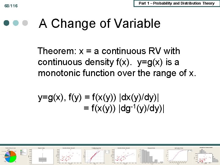
68/116 Part 1 – Probability and Distribution Theory A Change of Variable Theorem: x = a continuous RV with continuous density f(x). y=g(x) is a monotonic function over the range of x. y=g(x), f(y) = f(x(y)) |dx(y)/dy)| = f(x(y)) |dg-1(y)/dy)|
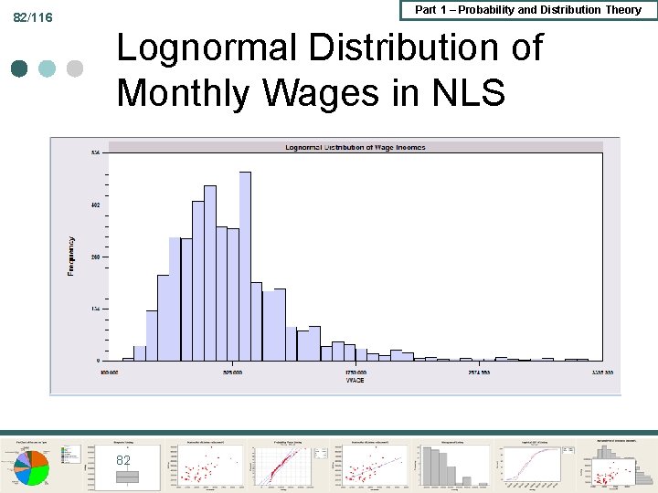
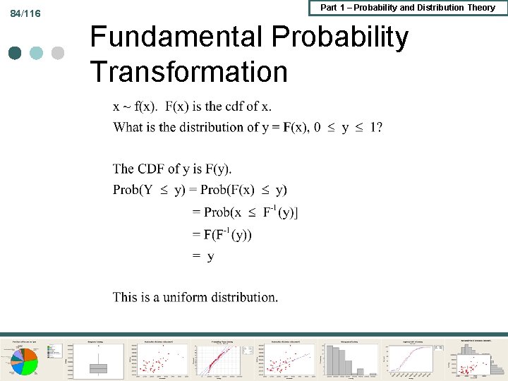
Part 1 – Probability and Distribution Theory 69/116 Change of Variable Applications ¢ Standardized normal ¢ Lognormal to normal ¢ Fundamental probability transform Random number generators, science and encryption
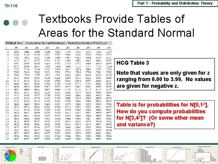
70/116 Part 1 – Probability and Distribution Theory Textbooks Provide Tables of Areas for the Standard Normal HCG Table 3 Note that values are only given for z ranging from 0. 00 to 3. 99. No values are given for negative z. Table is for probabilities for N[0, 12]. How do you compute probabilities for N[3, 42]? (Or some other mean and variance? )
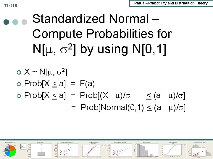
71/116 Part 1 – Probability and Distribution Theory Standardized Normal – Compute Probabilities for 2 N[ , ] by using N[0, 1] ¢ ¢ ¢ X ~ N[ , 2] Prob[X < a] = F(a) Prob[X < a] = Prob[(X - )/ < (a - )/ ] = Prob[Normal(0, 1) < (a - )/ ]
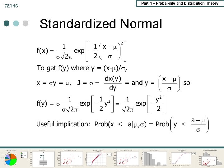
Part 1 – Probability and Distribution Theory 72/116 Standardized Normal 72
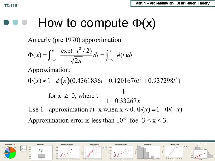
Part 1 – Probability and Distribution Theory 73/116 How to compute (x) 73
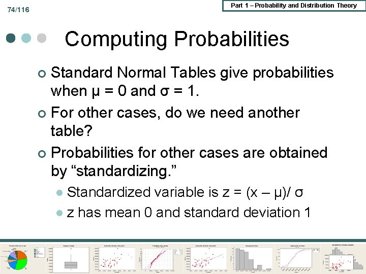
Part 1 – Probability and Distribution Theory 74/116 Computing Probabilities Standard Normal Tables give probabilities when μ = 0 and σ = 1. ¢ For other cases, do we need another table? ¢ Probabilities for other cases are obtained by “standardizing. ” ¢ Standardized variable is z = (x – μ)/ σ l z has mean 0 and standard deviation 1 l
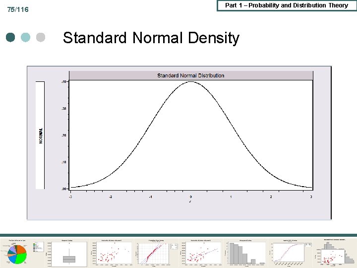
75/116 Part 1 – Probability and Distribution Theory Standard Normal Density
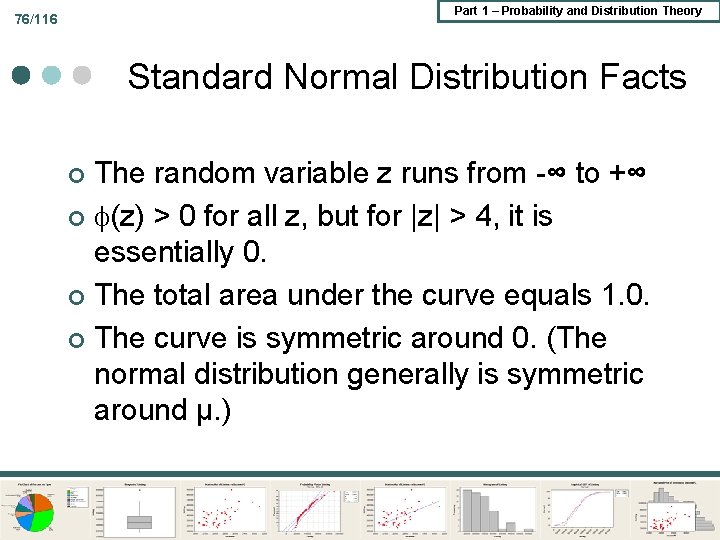
Part 1 – Probability and Distribution Theory 76/116 Standard Normal Distribution Facts The random variable z runs from -∞ to +∞ ¢ (z) > 0 for all z, but for |z| > 4, it is essentially 0. ¢ The total area under the curve equals 1. 0. ¢ The curve is symmetric around 0. (The normal distribution generally is symmetric around μ. ) ¢
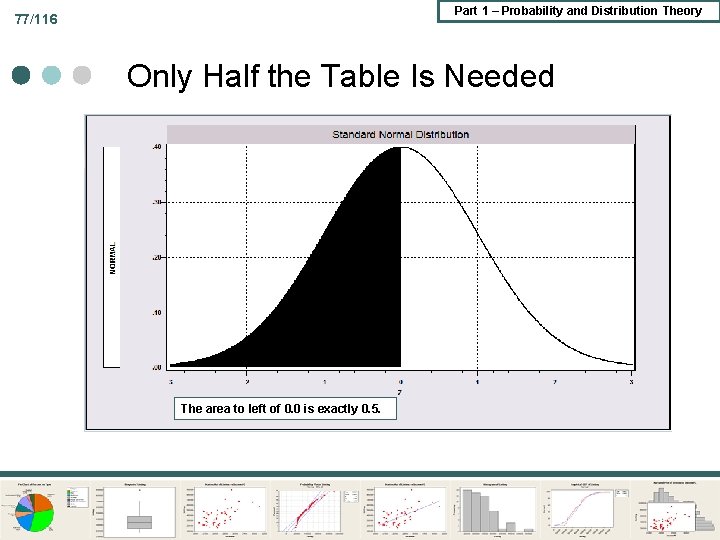
Part 1 – Probability and Distribution Theory 77/116 Only Half the Table Is Needed The area to left of 0. 0 is exactly 0. 5.
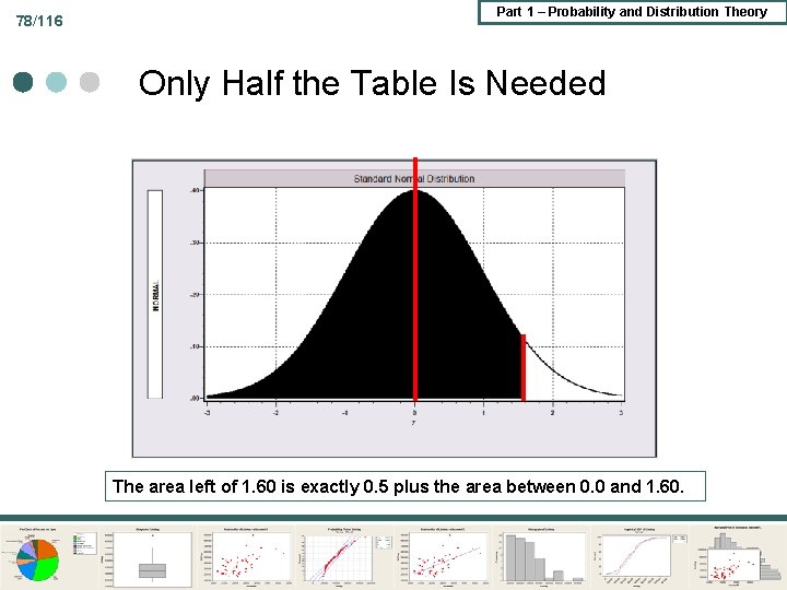
78/116 Part 1 – Probability and Distribution Theory Only Half the Table Is Needed The area left of 1. 60 is exactly 0. 5 plus the area between 0. 0 and 1. 60.
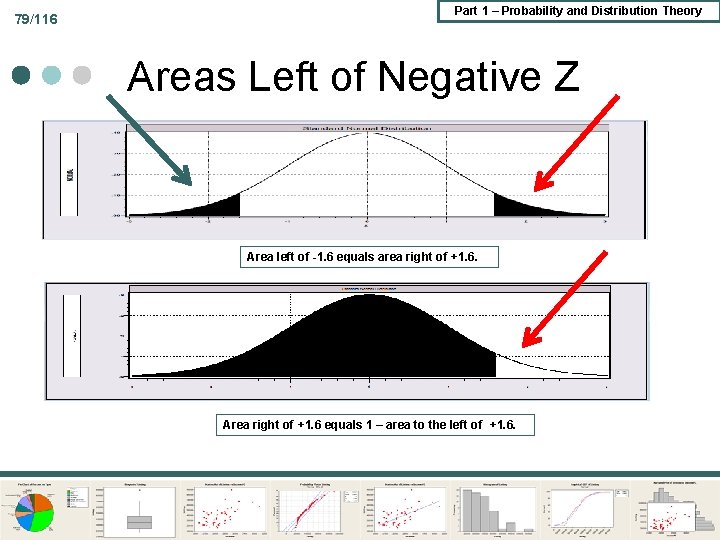
79/116 Part 1 – Probability and Distribution Theory Areas Left of Negative Z Area left of -1. 6 equals area right of +1. 6. Area right of +1. 6 equals 1 – area to the left of +1. 6.
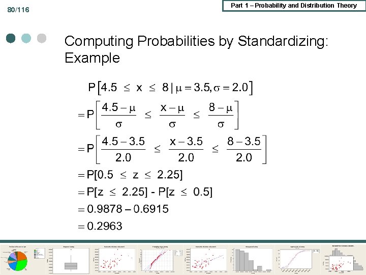
80/116 Part 1 – Probability and Distribution Theory Computing Probabilities by Standardizing: Example
81/116 Part 1 – Probability and Distribution Theory Lognormal Distribution
Part 1 – Probability and Distribution Theory 82/116 Lognormal Distribution of Monthly Wages in NLS 82

Part 1 – Probability and Distribution Theory 83/116 Log of Lognormal Variable 83
84/116 Part 1 – Probability and Distribution Theory Fundamental Probability Transformation
Part 1 – Probability and Distribution Theory 85/116 Random Number Generation The CDF is a monotonic function of x ¢ If u = F(x), x = F-1(u) ¢ We can generate u with a computer ¢ Example: Exponential l Example: Normal l

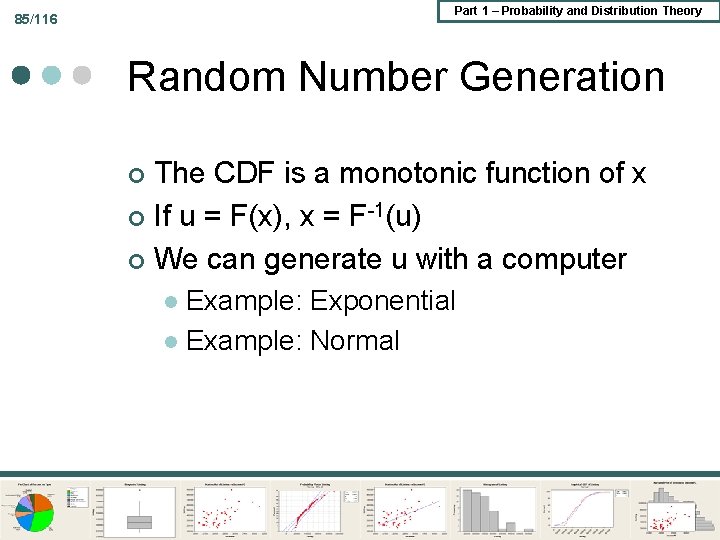
Part 1 – Probability and Distribution Theory 86/116 Generating Random Samples ¢ Exponential u = F(x) = 1 – exp(- x) l 1 – u = exp(- x) l x = (-1/ ) ln(1 – u) l ¢ Normal ( , ) u = (z) l z = -1(u) l x = z + = -1(u) + l
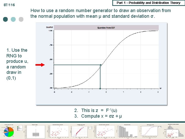
87/116 Part 1 – Probability and Distribution Theory How to use a random number generator to draw an observation from the normal population with mean μ and standard deviation σ. 1. Use the RNG to produce u, a random draw in (0, 1) 2. This is z = F-1(u) 3. Compute x = σz + μ
![Part 1 – Probability and Distribution Theory 88/116 U[0, 1] Generation Linear congruential generator Part 1 – Probability and Distribution Theory 88/116 U[0, 1] Generation Linear congruential generator](http://slidetodoc.com/presentation_image_h2/6c82ac49934e1f40d3ce2dc40316f335/image-88.jpg)
Part 1 – Probability and Distribution Theory 88/116 U[0, 1] Generation Linear congruential generator x(n) = (a x(n-1) + b)mod m ¢ Properties of RNGs ¢ Replicability – they are not RANDOM l Period l Randomness tests l ¢ The Mersenne twister: Current state of the art (of pseudo-random number generation)
Part 1 – Probability and Distribution Theory 89/116 Nonsense. He didn’t. 89

Part 1 – Probability and Distribution Theory 3 – Joint Distributions

91/116 Part 1 – Probability and Distribution Theory Jointly Distributed Random Variables Usually some kind of association between the variables. E. g. , two different financial assets Joint cdf for two random variables F(x, y) = Prob(X < x, Y < y)
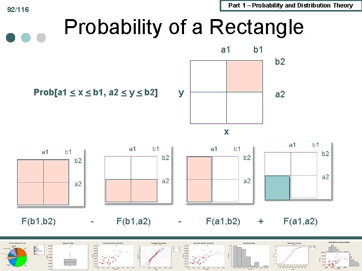
Part 1 – Probability and Distribution Theory 92/116 Probability of a Rectangle a 1 b 2 Prob[a 1 < x < b 1, a 2 < y < b 2] y a 2 x F(b 1, b 2) - F(b 1, a 2) - F(a 1, b 2) + F(a 1, a 2)
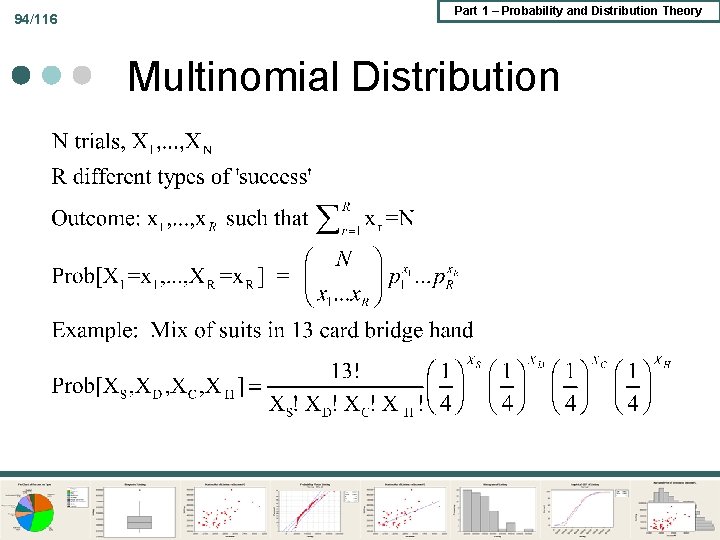
Part 1 – Probability and Distribution Theory 93/116 Joint Distributions ¢ Discrete: Multinomial for R kinds of success in N independent trials ¢ Continuous: Bi- and Multivariate normal ¢ Mixed: Conditional regression models
94/116 Part 1 – Probability and Distribution Theory Multinomial Distribution
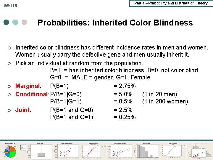
95/116 Part 1 – Probability and Distribution Theory Probabilities: Inherited Color Blindness ¢ ¢ ¢ Inherited color blindness has different incidence rates in men and women. Women usually carry the defective gene and men usually inherit it. Pick an individual at random from the population. B=1 = has inherited color blindness, B=0, not color blind G=0 = MALE = gender, G=1, Female Marginal: P(B=1) = 2. 75% Conditional: P(B=1|G=0) = 5. 0% (1 in 20 men) P(B=1|G=1) = 0. 5% (1 in 200 women) Joint: P(B=1 and G=0) = 2. 5% P(B=1 and G=1) = 0. 25%
![Part 1 – Probability and Distribution Theory 96/116 Marginal Distributions Prob[X=x] = y Prob[X=x, Part 1 – Probability and Distribution Theory 96/116 Marginal Distributions Prob[X=x] = y Prob[X=x,](http://slidetodoc.com/presentation_image_h2/6c82ac49934e1f40d3ce2dc40316f335/image-96.jpg)
Part 1 – Probability and Distribution Theory 96/116 Marginal Distributions Prob[X=x] = y Prob[X=x, Y=y] Color Blind Gender B=0 B=1 Total G=0 . 475 . 025 0. 50 G=1 . 4975 . 0025 0. 50 Total . 97255 . 0275 1. 00 Prob[G=0]=Prob[G=0, B=0]+ Prob[G=0, B=1]

97/116 Part 1 – Probability and Distribution Theory Joint Continuous Distribution
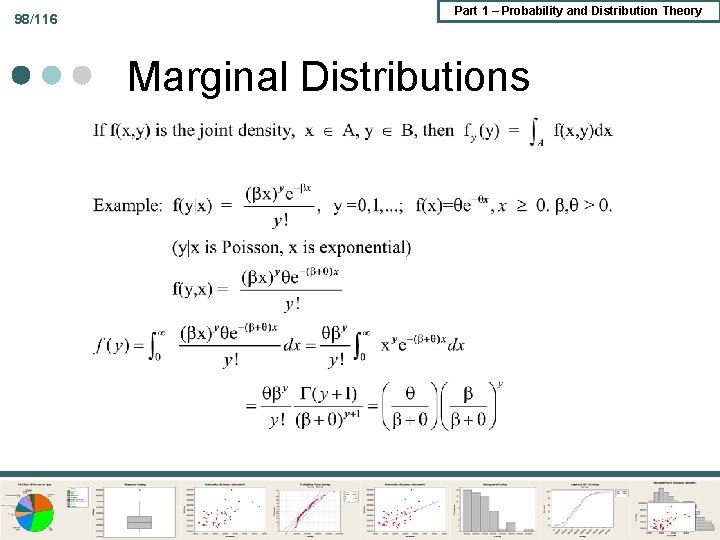
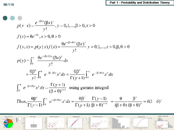
98/116 Part 1 – Probability and Distribution Theory Marginal Distributions
99/116 Part 1 – Probability and Distribution Theory
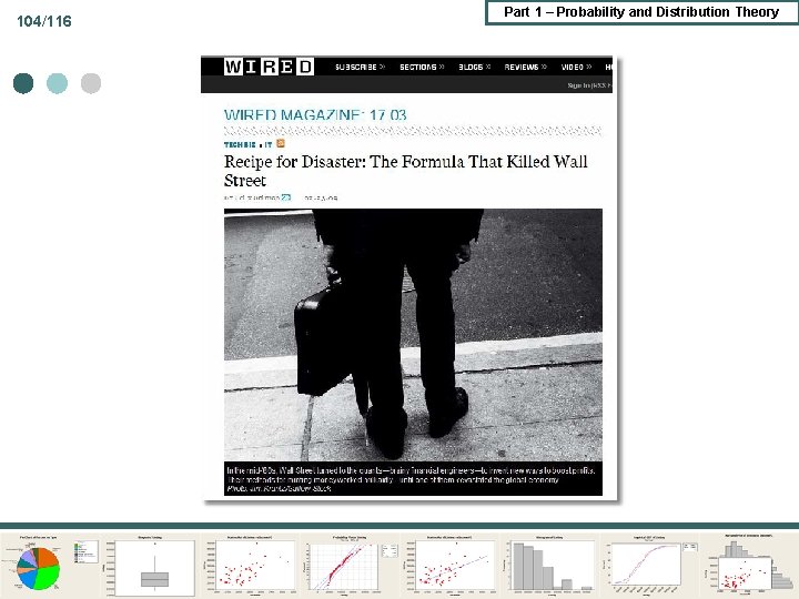
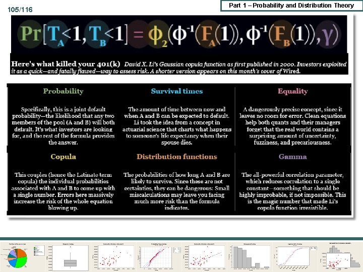
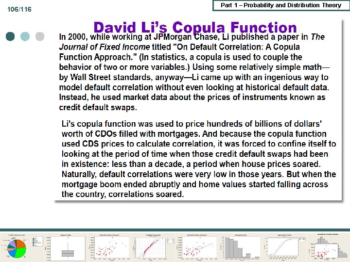
Part 1 – Probability and Distribution Theory 100/116 Two Leading Applications of Joint Distributions ¢ Copula Function - Application in Finance ¢ Bivariate Normal Distribution
101/116 Part 1 – Probability and Distribution Theory
102/116 Part 1 – Probability and Distribution Theory
103/116 Part 1 – Probability and Distribution Theory
104/116 Part 1 – Probability and Distribution Theory
105/116 Part 1 – Probability and Distribution Theory
106/116 Part 1 – Probability and Distribution Theory
107/116 Part 1 – Probability and Distribution Theory
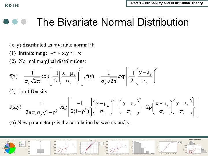
108/116 Part 1 – Probability and Distribution Theory The Bivariate Normal Distribution
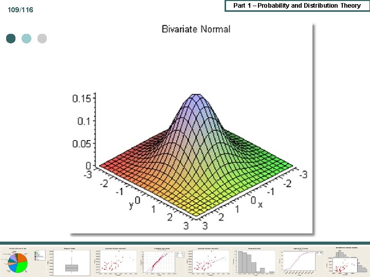
109/116 Part 1 – Probability and Distribution Theory
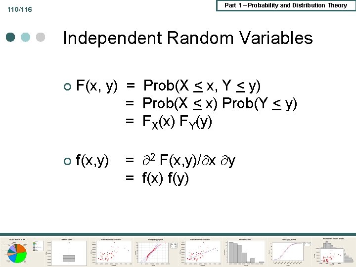
Part 1 – Probability and Distribution Theory 110/116 Independent Random Variables ¢ F(x, y) = Prob(X < x, Y < y) = Prob(X < x) Prob(Y < y) = FX(x) FY(y) ¢ f(x, y) = 2 F(x, y)/ x y = f(x) f(y)
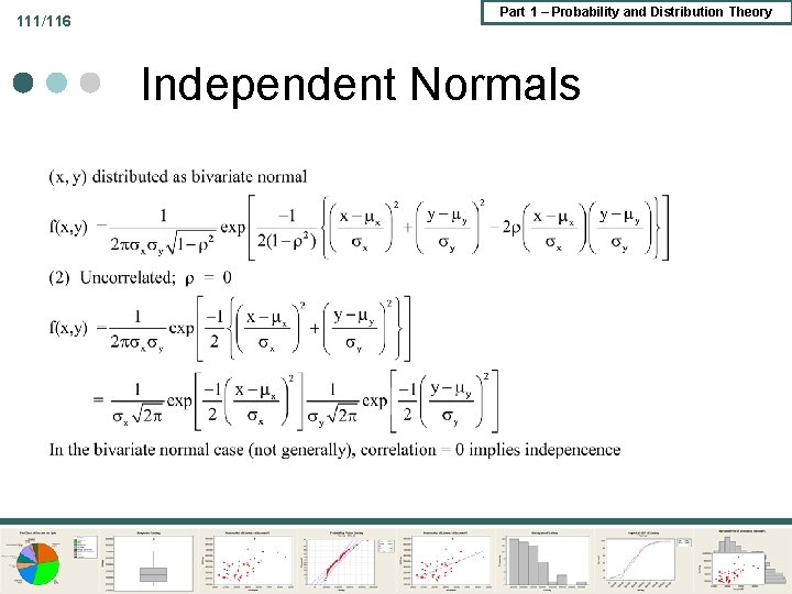
111/116 Part 1 – Probability and Distribution Theory Independent Normals
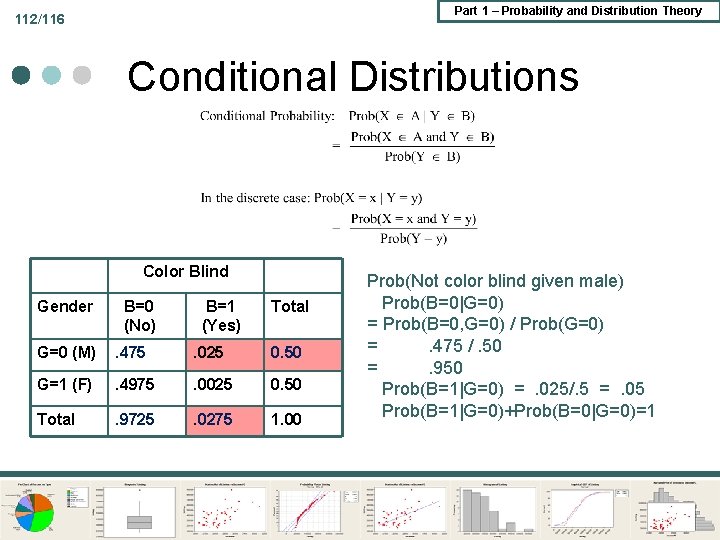
Part 1 – Probability and Distribution Theory 112/116 Conditional Distributions Color Blind Gender B=0 (No) B=1 (Yes) Total G=0 (M) . 475 . 025 0. 50 G=1 (F) . 4975 . 0025 0. 50 Total . 97255 . 0275 1. 00 Prob(Not color blind given male) Prob(B=0|G=0) = Prob(B=0, G=0) / Prob(G=0) =. 475 /. 50 =. 950 Prob(B=1|G=0) =. 025/. 5 =. 05 Prob(B=1|G=0)+Prob(B=0|G=0)=1
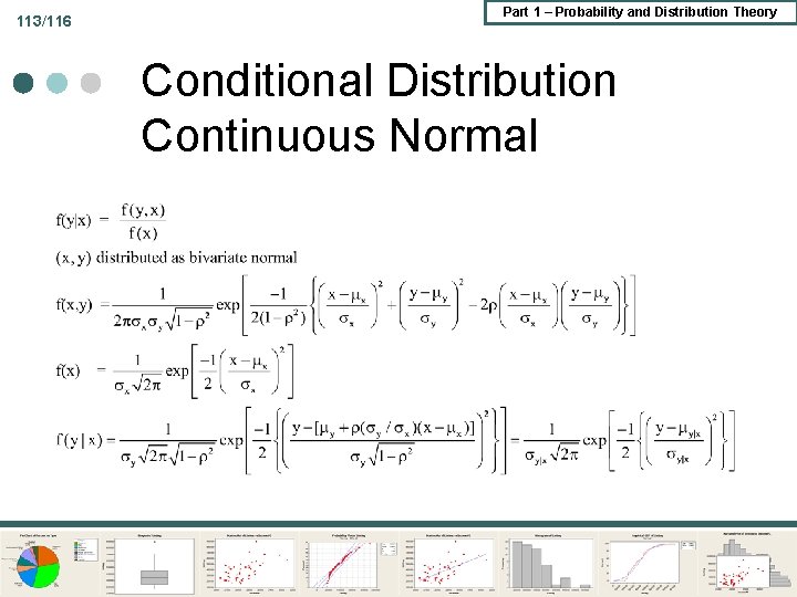
113/116 Part 1 – Probability and Distribution Theory Conditional Distribution Continuous Normal
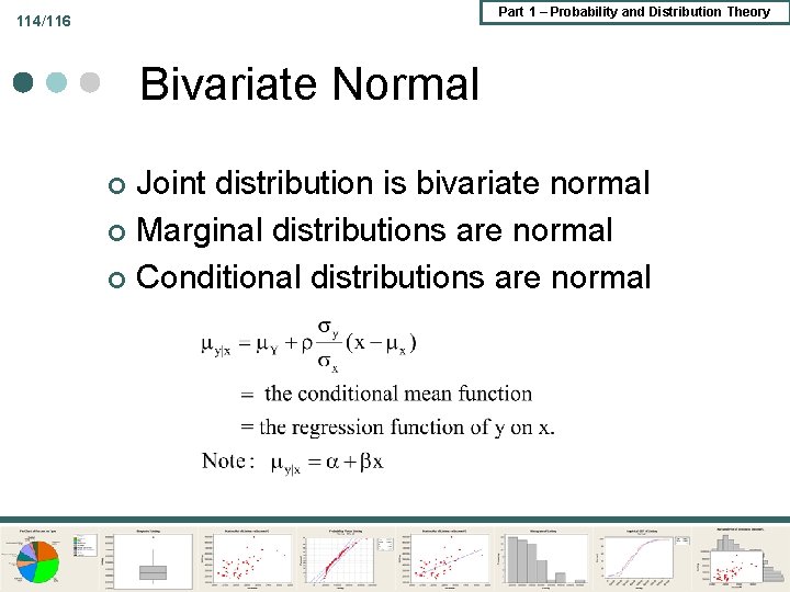
Part 1 – Probability and Distribution Theory 114/116 Bivariate Normal Joint distribution is bivariate normal ¢ Marginal distributions are normal ¢ Conditional distributions are normal ¢
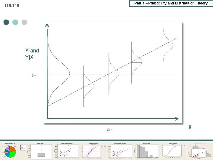
Part 1 – Probability and Distribution Theory 115/116 Y and Y|X Y X X
Part 1 – Probability and Distribution Theory 116/116 Model Building ¢ ¢ Typically f(y|x) is of interest x is generated by a separate process f(x) Joint distribution is f(y, x)=f(y|x)f(x) Ex: demographic y = log(household income|family size) x = family size l y|x ~ Normal( y|x , y|x ) l x ~ Poisson ( )
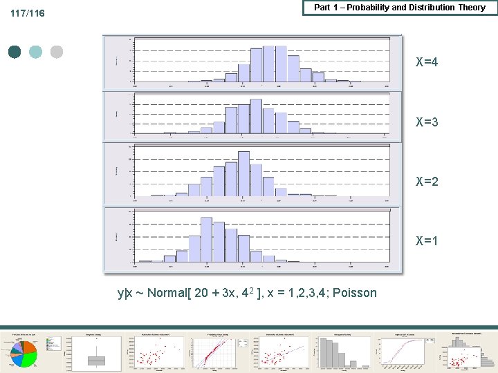
117/116 Part 1 – Probability and Distribution Theory X=4 X=3 X=2 X=1 y|x ~ Normal[ 20 + 3 x, 42 ], x = 1, 2, 3, 4; Poisson
- Slides: 117