PARAMETRIC LINEAR PROGRAMMING We have considered the sensitivity

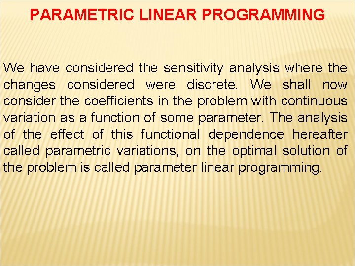
PARAMETRIC LINEAR PROGRAMMING We have considered the sensitivity analysis where the changes considered were discrete. We shall now consider the coefficients in the problem with continuous variation as a function of some parameter. The analysis of the effect of this functional dependence hereafter called parametric variations, on the optimal solution of the problem is called parameter linear programming.

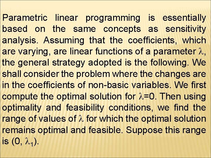
Parametric linear programming is essentially based on the same concepts as sensitivity analysis. Assuming that the coefficients, which are varying, are linear functions of a parameter , the general strategy adopted is the following. We shall consider the problem where the changes are in the coefficients of non-basic variables. We first compute the optimal solution for =0. Then using optimality and feasibility conditions, we find the range of values of for which the optimal solution remains optimal and feasible. Suppose this range is (0, 1).

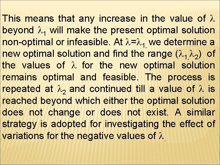
This means that any increase in the value of beyond 1 will make the present optimal solution non-optimal or infeasible. At = 1, we determine a new optimal solution and find the range ( 1, 2) of the values of for the new optimal solution remains optimal and feasible. The process is repeated at 2 and continued till a value of is reached beyond which either the optimal solution does not change or does not exist. A similar strategy is adopted for investigating the effect of variations for the negative values of .

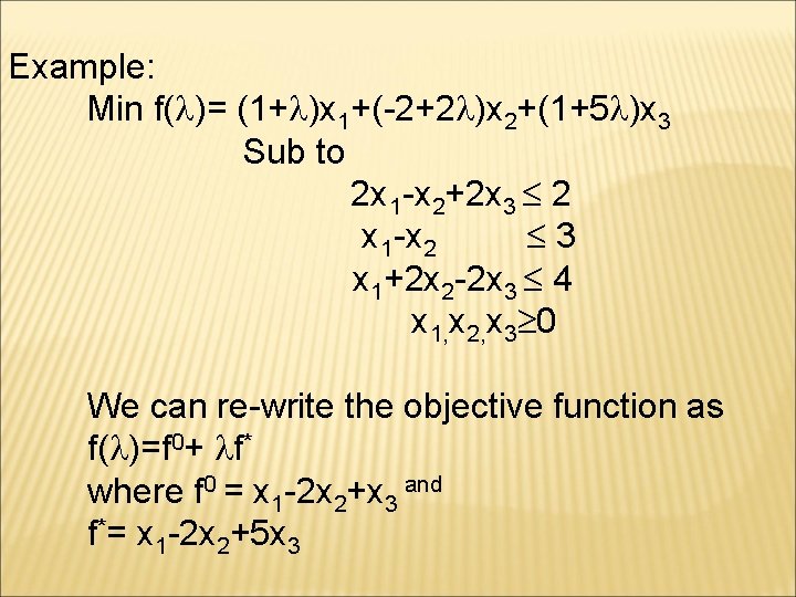
Example: Min f( )= (1+ )x 1+(-2+2 )x 2+(1+5 )x 3 Sub to 2 x 1 -x 2+2 x 3 2 x 1 -x 2 3 x 1+2 x 2 -2 x 3 4 x 1, x 2, x 3 0 We can re-write the objective function as f( )=f 0+ f* where f 0 = x 1 -2 x 2+x 3 and f*= x 1 -2 x 2+5 x 3

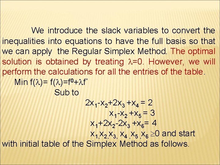
We introduce the slack variables to convert the inequalities into equations to have the full basis so that we can apply the Regular Simplex Method. The optimal solution is obtained by treating =0. However, we will perform the calculations for all the entries of the table. Min f( )=f 0+ f* Sub to 2 x 1 -x 2+2 x 3 +x 4 = 2 x 1 -x 2 +x 5 = 3 x 1+2 x 2 -2 x 3 +x 6= 4 x 1, x 2, x 3, x 4 , x 5 , x 6 0 and start with initial table of the Simplex Method as follows.

Step II: We set up an initial table as: Cb c* j→ 1 -2 5 0 0 0 Cj→ 1 -2 1 0 0 0 Ratios b f* f 0 Xb↓ y 1 y 2 y 3 y 4 y 5 y 6 0 0 x 4 2 -1 2 1 0 0 2 0 0 x 5 1 -1 0 0 1 0 3 0 0 x 6 1 2 -2 0 0 1 4 Zj-Cj(f 0) -1 2 1 0 0 0 Z=0 Zj--Cj(f*) -1 2 -5 0 0 0 Z=0 4/2=2

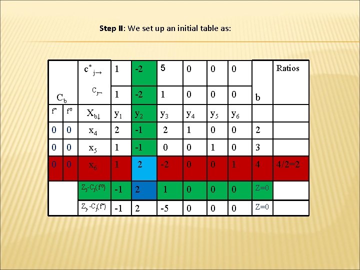
Step II: We set up an initial table as: Cb c* j→ 1 -2 5 0 0 0 Cj→ 1 -2 1 0 0 0 y 4 y 5 y 6 Ratios b f* f 0 Xb↓ y 1 y 2 y 3 0 0 x 4 5/2 0 1 1 0 1/2 4 0 0 x 5 3/2 0 -1 0 1 1/2 5 -2 -2 x 2 1/2 1 -1 0 0 1/2 2 Zj-Cj(f 0) -2 0 1 0 0 -1 Z=-4 Zj--Cj(f*) -2 0 -3 0 0 -1 Z=-4 4/1=4

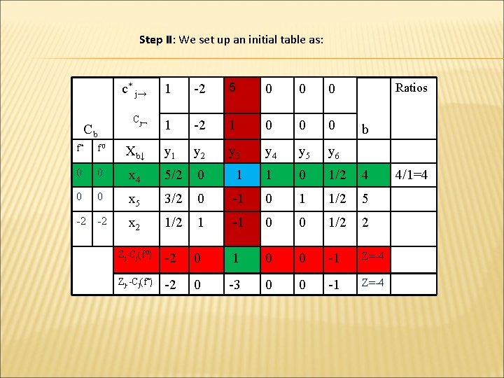
Step II: We set up an initial table as: Cb c* j→ 1 -2 5 0 0 0 Cj→ 1 -2 1 0 0 0 y 4 y 5 y 6 Ratios b f* f 0 Xb↓ y 1 y 2 y 3 5 1 x 3 5/2 0 1 1 0 1/2 4 0 0 x 5 4 0 0 1 1 1 9 -2 -2 x 2 3 1 0 1 6 Zj-Cj(f 0) -9/2 0 1 0 0 -3/2 Z=-8 Zj--Cj(f*) 11/2 0 3 0 0 1/2 Z=-8 4/1=4

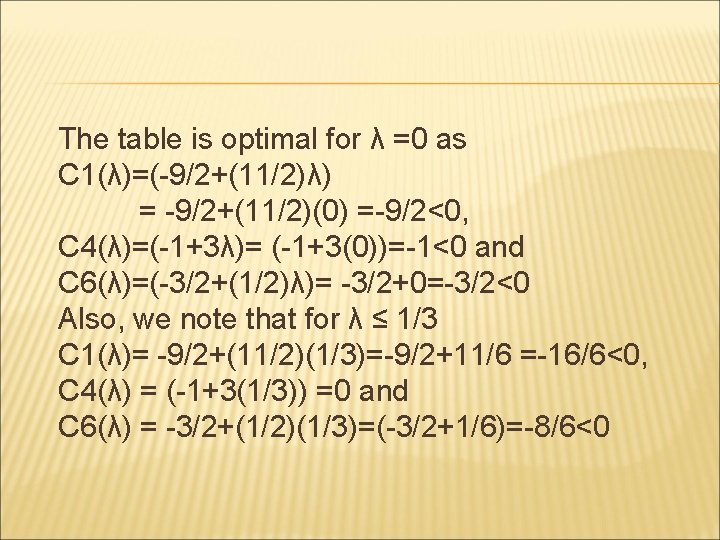
The table is optimal for λ =0 as C 1(λ)=(-9/2+(11/2)λ) = -9/2+(11/2)(0) =-9/2<0, C 4(λ)=(-1+3λ)= (-1+3(0))=-1<0 and C 6(λ)=(-3/2+(1/2)λ)= -3/2+0=-3/2<0 Also, we note that for λ ≤ 1/3 C 1(λ)= -9/2+(11/2)(1/3)=-9/2+11/6 =-16/6<0, C 4(λ) = (-1+3(1/3)) =0 and C 6(λ) = -3/2+(1/2)(1/3)=(-3/2+1/6)=-8/6<0

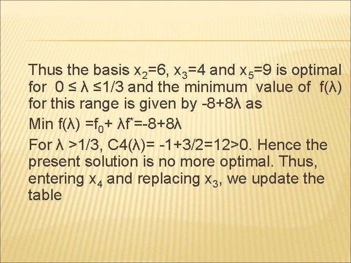
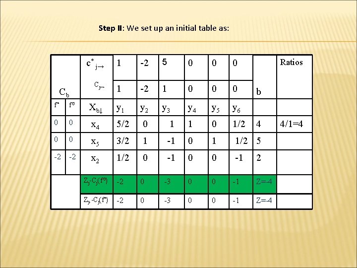
Thus the basis x 2=6, x 3=4 and x 5=9 is optimal for 0 ≤ λ ≤ 1/3 and the minimum value of f(λ) for this range is given by -8+8λ as Min f(λ) =f 0+ λf*=-8+8λ For λ >1/3, C 4(λ)= -1+3/2=12>0. Hence the present solution is no more optimal. Thus, entering x 4 and replacing x 3, we update the table

Step II: We set up an initial table as: Cb c* j→ 1 -2 5 0 0 0 Cj→ 1 -2 1 0 0 0 y 3 y 4 y 5 y 6 Ratios b f* f 0 Xb↓ y 1 y 2 0 0 x 4 5/2 0 1 1 0 1/2 0 0 x 5 3/2 1 -1 0 1 1/2 5 -2 -2 x 2 1/2 0 -1 0 0 -1 4 2 Zj-Cj(f 0) -2 0 -3 0 0 -1 Z=-4 Zj--Cj(f*) -2 0 -3 0 0 -1 Z=-4 4/1=4

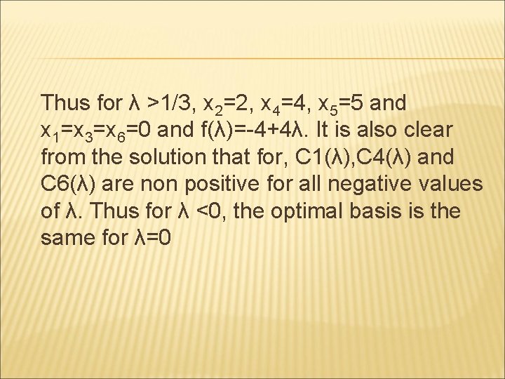
Thus for λ >1/3, x 2=2, x 4=4, x 5=5 and x 1=x 3=x 6=0 and f(λ)=-4+4λ. It is also clear from the solution that for, C 1(λ), C 4(λ) and C 6(λ) are non positive for all negative values of λ. Thus for λ <0, the optimal basis is the same for λ=0