Parametric Curves Surfaces What is a parametric curve

Parametric Curves & Surfaces

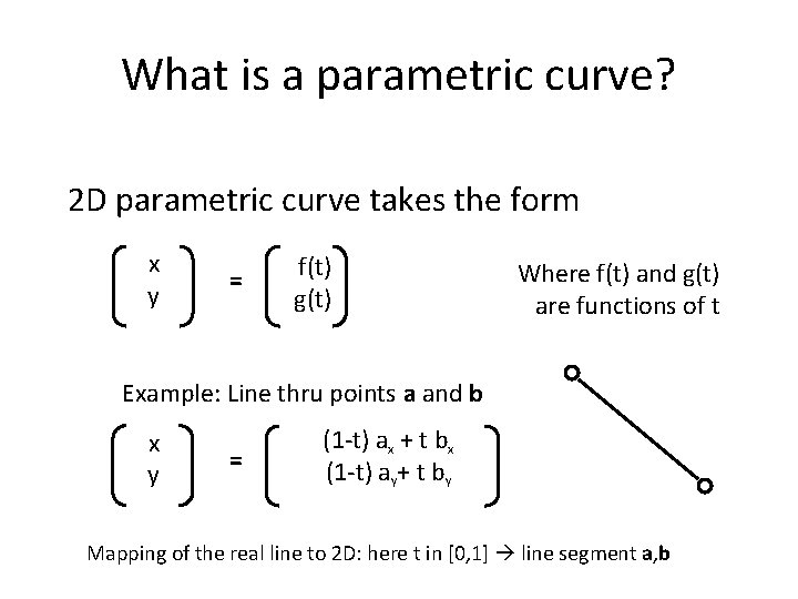
What is a parametric curve? 2 D parametric curve takes the form x y = f(t) g(t) Where f(t) and g(t) are functions of t Example: Line thru points a and b x y = (1 -t) ax + t bx (1 -t) ay+ t by Mapping of the real line to 2 D: here t in [0, 1] line segment a, b

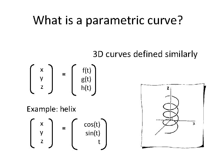
What is a parametric curve? 3 D curves defined similarly x y z = f(t) g(t) h(t) Example: helix x y z = cos(t) sin(t) t

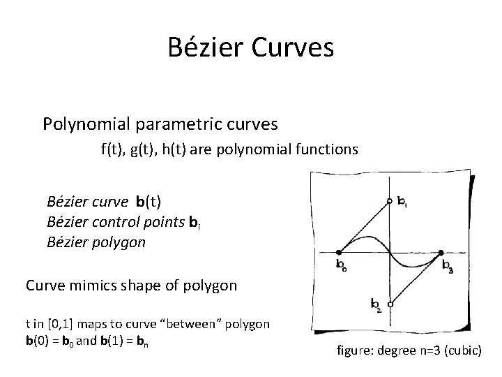
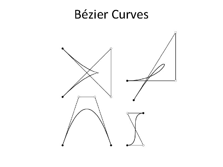
Bézier Curves Polynomial parametric curves f(t), g(t), h(t) are polynomial functions Bézier curve b(t) Bézier control points bi Bézier polygon Curve mimics shape of polygon t in [0, 1] maps to curve “between” polygon b(0) = b 0 and b(1) = bn figure: degree n=3 (cubic)

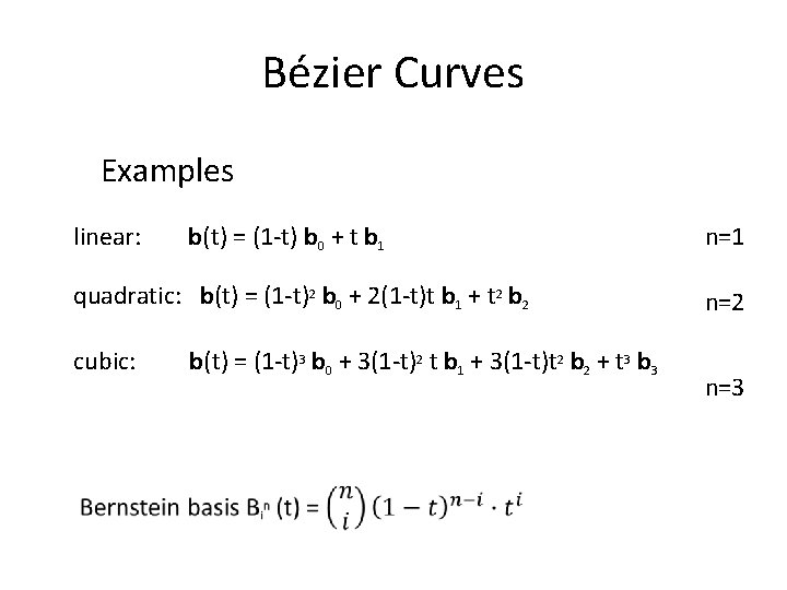
Bézier Curves Examples linear: b(t) = (1 -t) b 0 + t b 1 quadratic: b(t) = (1 -t)2 b 0 + 2(1 -t)t b 1 + t 2 b 2 cubic: b(t) = (1 -t)3 b 0 + 3(1 -t)2 t b 1 + 3(1 -t)t 2 b 2 + t 3 b 3 n=1 n=2 n=3

Bézier Curves

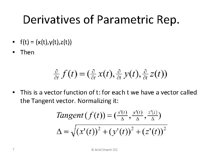
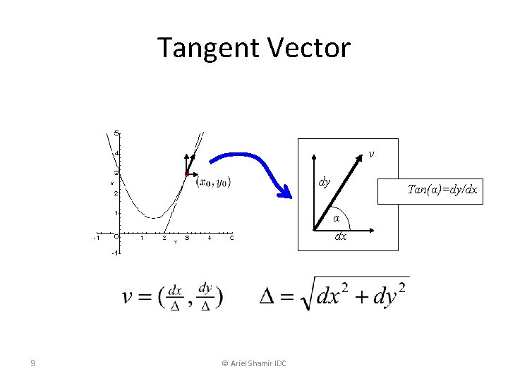
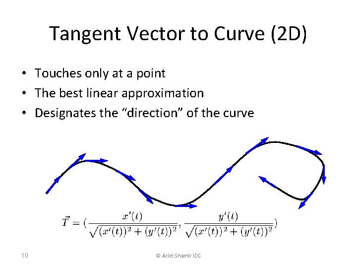
Derivatives of Parametric Rep. • f(t) = (x(t), y(t), z(t)) • Then • This is a vector function of t: for each t we have a vector called the Tangent vector. Normalizing it: 7 © Ariel Shamir IDC

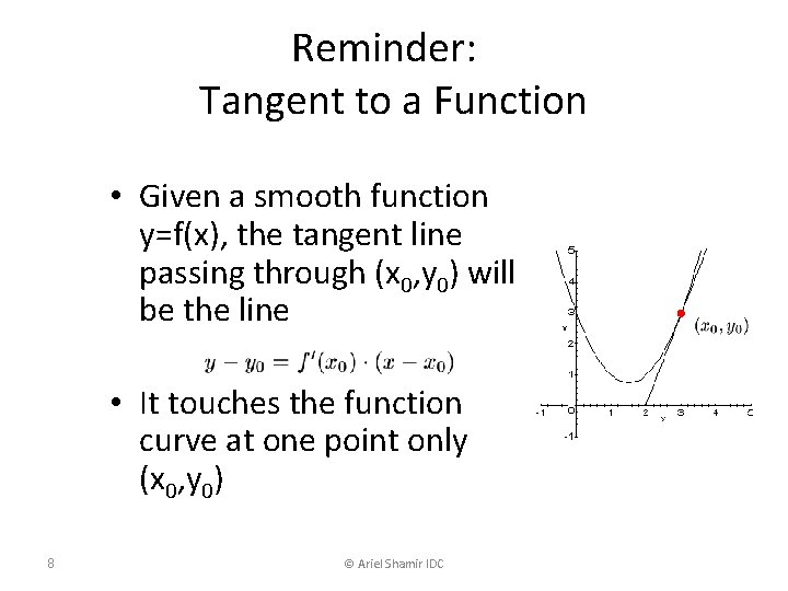
Reminder: Tangent to a Function • Given a smooth function y=f(x), the tangent line passing through (x 0, y 0) will be the line • It touches the function curve at one point only (x 0, y 0) 8 © Ariel Shamir IDC

Tangent Vector v dy Tan(α)=dy/dx α dx 9 © Ariel Shamir IDC

Tangent Vector to Curve (2 D) • Touches only at a point • The best linear approximation • Designates the “direction” of the curve 10 © Ariel Shamir IDC

Normal to the Curve (2 D) 11 © Ariel Shamir IDC

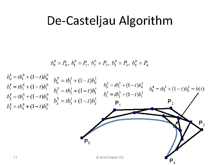
De-Casteljau Algorithm P 1 P 2 P 3 P 0 12 © Ariel Shamir IDC P 4

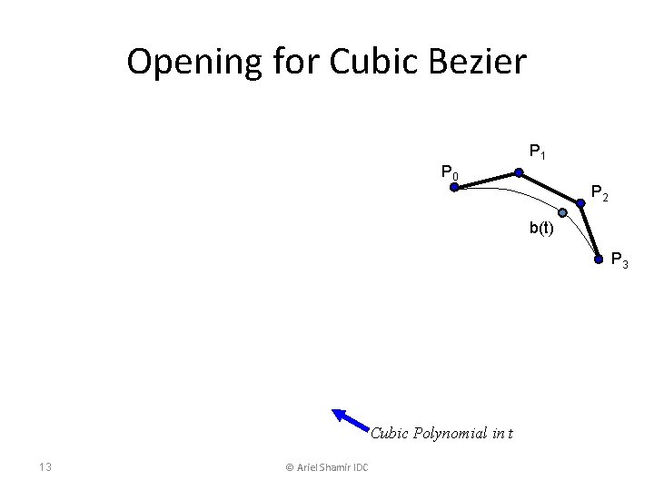
Opening for Cubic Bezier P 0 P 1 P 2 b(t) P 3 Cubic Polynomial in t 13 © Ariel Shamir IDC

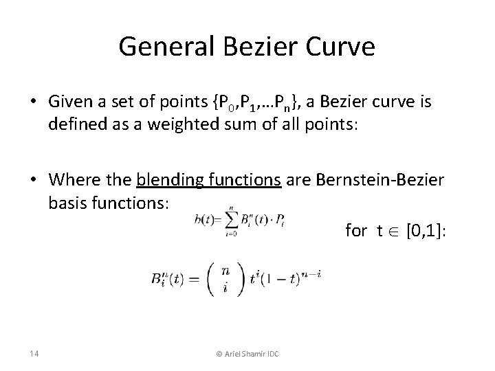
General Bezier Curve • Given a set of points {P 0, P 1, …Pn}, a Bezier curve is defined as a weighted sum of all points: • Where the blending functions are Bernstein-Bezier basis functions: for t [0, 1]: 14 © Ariel Shamir IDC

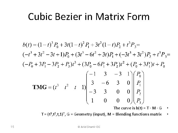
Cubic Bezier in Matrix Form The curve is b(t) = T · M · G T = (t 3, t 2, t, 1)T, G = Geometry (input), M = Blending functions matrix 15 © Ariel Shamir IDC • •

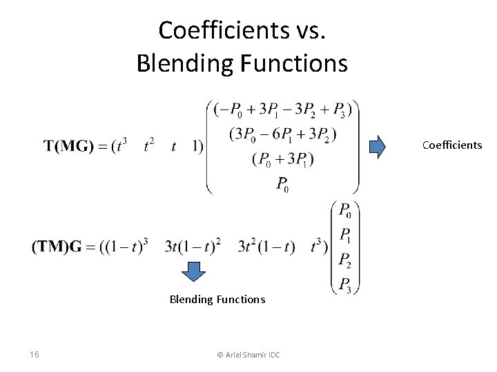
Coefficients vs. Blending Functions Coefficients Blending Functions 16 © Ariel Shamir IDC

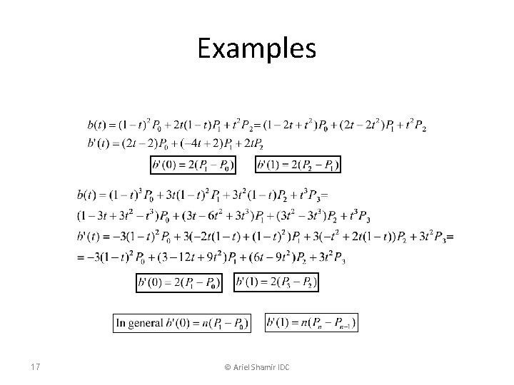
Examples 17 © Ariel Shamir IDC

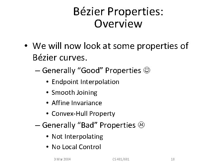
Bézier Properties: Overview • We will now look at some properties of Bézier curves. – Generally “Good” Properties • • Endpoint Interpolation Smooth Joining Affine Invariance Convex-Hull Property – Generally “Bad” Properties • Not Interpolating • No Local Control 3 Mar 2004 CS 481/681 18

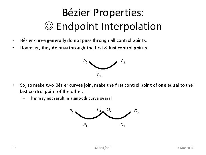
Bézier Properties: Endpoint Interpolation • • Bézier curve generally do not pass through all control points. However, they do pass through the first & last control points. P 0 P 2 P 1 • So, to make two Bézier curves join, make the first control point of one equal to the last control point of the other. – This may not result in a smooth curve overall. P 2 P 0 Q 0 P 1 19 Q 2 Q 1 CS 481/681 3 Mar 2004

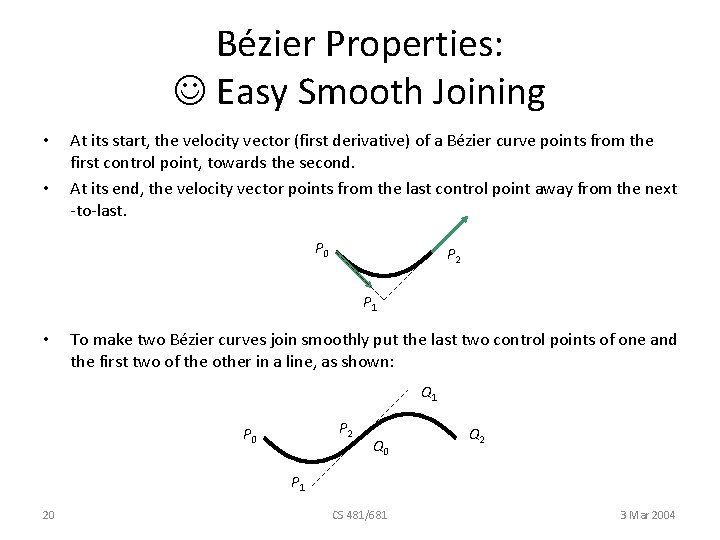
Bézier Properties: Easy Smooth Joining • • At its start, the velocity vector (first derivative) of a Bézier curve points from the first control point, towards the second. At its end, the velocity vector points from the last control point away from the next -to-last. P 0 P 2 P 1 • To make two Bézier curves join smoothly put the last two control points of one and the first two of the other in a line, as shown: Q 1 P 2 P 0 Q 2 P 1 20 CS 481/681 3 Mar 2004

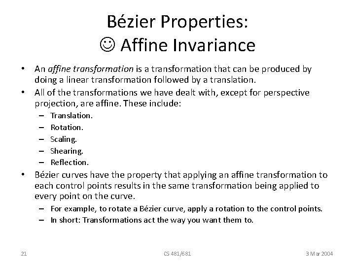
Bézier Properties: Affine Invariance • An affine transformation is a transformation that can be produced by doing a linear transformation followed by a translation. • All of the transformations we have dealt with, except for perspective projection, are affine. These include: – – – Translation. Rotation. Scaling. Shearing. Reflection. • Bézier curves have the property that applying an affine transformation to each control points results in the same transformation being applied to every point on the curve. – For example, to rotate a Bézier curve, apply a rotation to the control points. – In short: Transformations act the way you want them to. 21 CS 481/681 3 Mar 2004

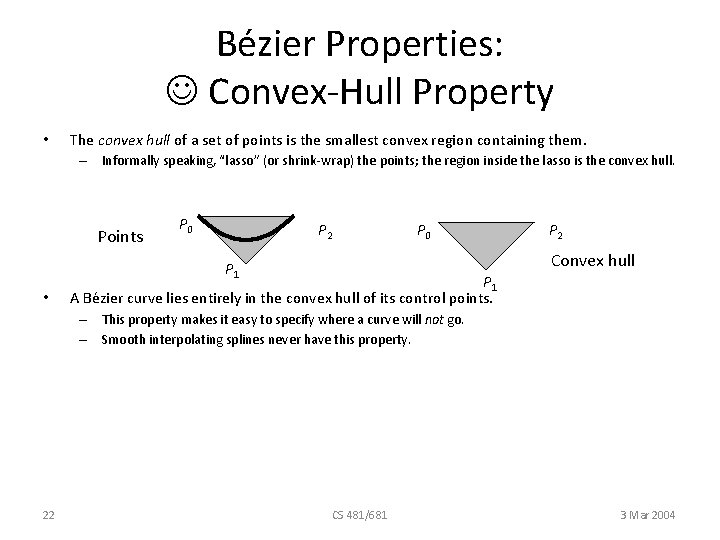
Bézier Properties: Convex-Hull Property • The convex hull of a set of points is the smallest convex region containing them. – Informally speaking, “lasso” (or shrink-wrap) the points; the region inside the lasso is the convex hull. Points P 0 P 2 P 0 Convex hull P 1 • P 2 P 1 A Bézier curve lies entirely in the convex hull of its control points. – This property makes it easy to specify where a curve will not go. – Smooth interpolating splines never have this property. 22 CS 481/681 3 Mar 2004

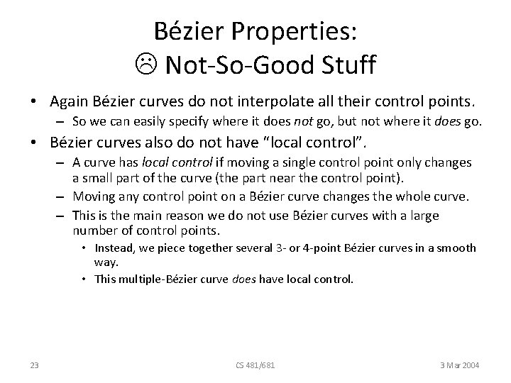
Bézier Properties: Not-So-Good Stuff • Again Bézier curves do not interpolate all their control points. – So we can easily specify where it does not go, but not where it does go. • Bézier curves also do not have “local control”. – A curve has local control if moving a single control point only changes a small part of the curve (the part near the control point). – Moving any control point on a Bézier curve changes the whole curve. – This is the main reason we do not use Bézier curves with a large number of control points. • Instead, we piece together several 3 - or 4 -point Bézier curves in a smooth way. • This multiple-Bézier curve does have local control. 23 CS 481/681 3 Mar 2004

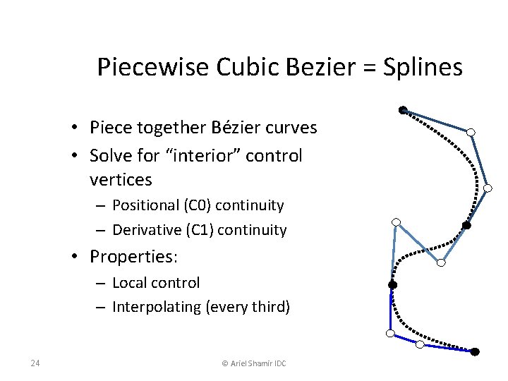
Piecewise Cubic Bezier = Splines • Piece together Bézier curves • Solve for “interior” control vertices – Positional (C 0) continuity – Derivative (C 1) continuity • Properties: – Local control – Interpolating (every third) 24 © Ariel Shamir IDC

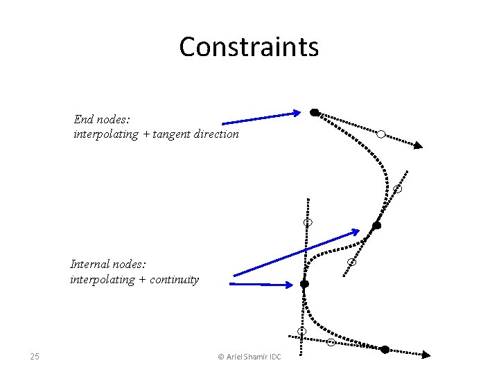
Constraints End nodes: interpolating + tangent direction Internal nodes: interpolating + continuity 25 © Ariel Shamir IDC

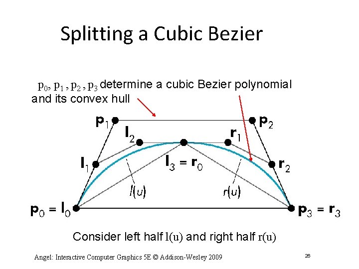
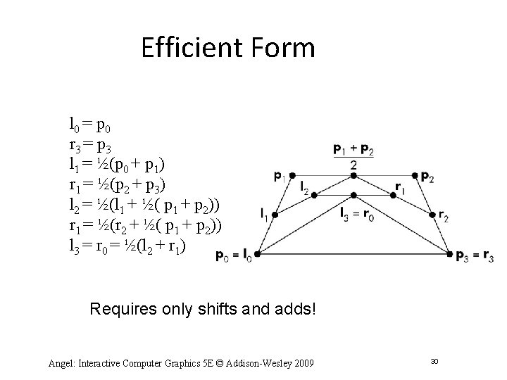
Splitting a Cubic Bezier p 0, p 1 , p 2 , p 3 determine a cubic Bezier polynomial and its convex hull Consider left half l(u) and right half r(u) Angel: Interactive Computer Graphics 5 E © Addison-Wesley 2009 26

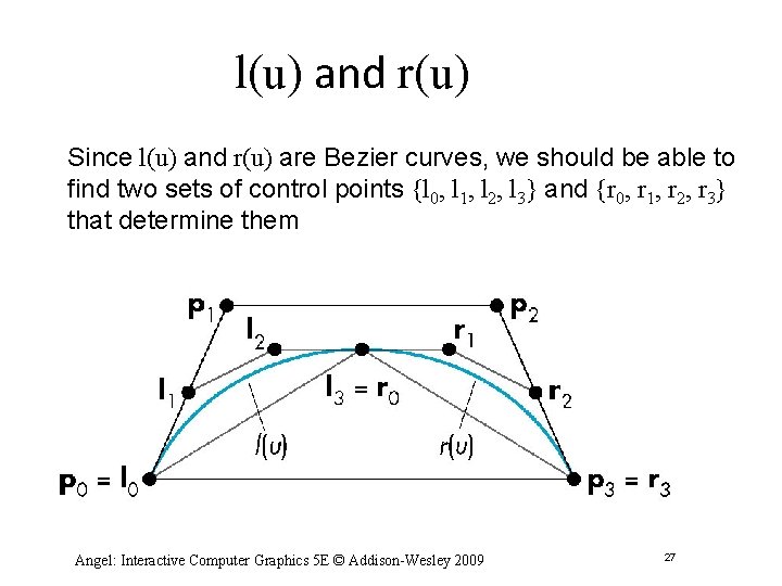
l(u) and r(u) Since l(u) and r(u) are Bezier curves, we should be able to find two sets of control points {l 0, l 1, l 2, l 3} and {r 0, r 1, r 2, r 3} that determine them Angel: Interactive Computer Graphics 5 E © Addison-Wesley 2009 27

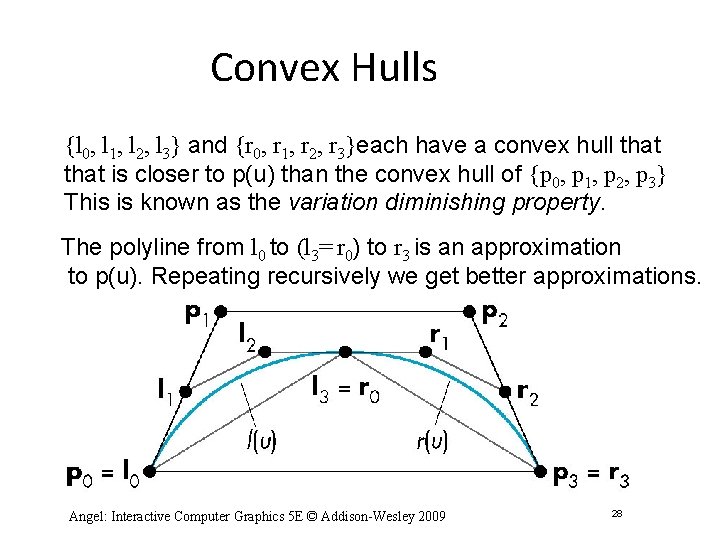
Convex Hulls {l 0, l 1, l 2, l 3} and {r 0, r 1, r 2, r 3}each have a convex hull that is closer to p(u) than the convex hull of {p 0, p 1, p 2, p 3} This is known as the variation diminishing property. The polyline from l 0 to (l 3= r 0) to r 3 is an approximation to p(u). Repeating recursively we get better approximations. Angel: Interactive Computer Graphics 5 E © Addison-Wesley 2009 28

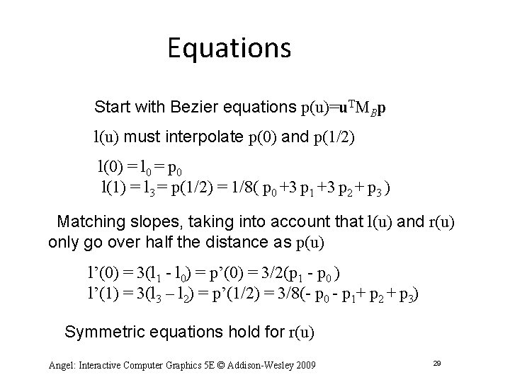
Equations Start with Bezier equations p(u)=u. TMBp l(u) must interpolate p(0) and p(1/2) l(0) = l 0 = p 0 l(1) = l 3 = p(1/2) = 1/8( p 0 +3 p 1 +3 p 2 + p 3 ) Matching slopes, taking into account that l(u) and r(u) only go over half the distance as p(u) l’(0) = 3(l 1 - l 0) = p’(0) = 3/2(p 1 - p 0 ) l’(1) = 3(l 3 – l 2) = p’(1/2) = 3/8(- p 0 - p 1+ p 2 + p 3) Symmetric equations hold for r(u) Angel: Interactive Computer Graphics 5 E © Addison-Wesley 2009 29

Efficient Form l 0 = p 0 r 3 = p 3 l 1 = ½(p 0 + p 1) r 1 = ½(p 2 + p 3) l 2 = ½(l 1 + ½( p 1 + p 2)) r 1 = ½(r 2 + ½( p 1 + p 2)) l 3 = r 0 = ½(l 2 + r 1) Requires only shifts and adds! Angel: Interactive Computer Graphics 5 E © Addison-Wesley 2009 30

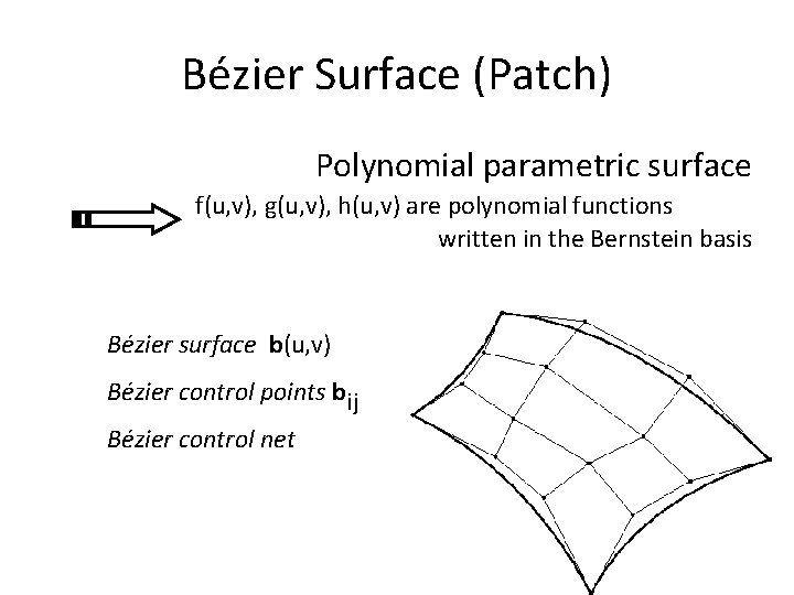
Bézier Surface (Patch) Polynomial parametric surface f(u, v), g(u, v), h(u, v) are polynomial functions written in the Bernstein basis Bézier surface b(u, v) Bézier control points bij Bézier control net

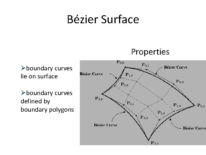
Bézier Surface Properties Øboundary curves lie on surface Øboundary curves defined by boundary polygons

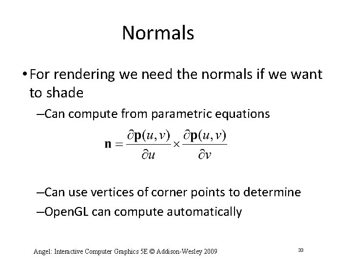
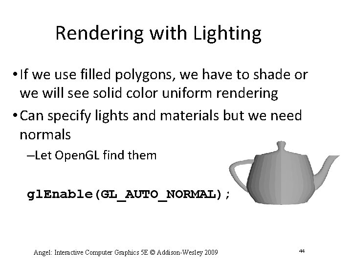
Normals • For rendering we need the normals if we want to shade –Can compute from parametric equations –Can use vertices of corner points to determine –Open. GL can compute automatically Angel: Interactive Computer Graphics 5 E © Addison-Wesley 2009 33

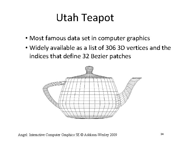
Utah Teapot • Most famous data set in computer graphics • Widely available as a list of 306 3 D vertices and the indices that define 32 Bezier patches Angel: Interactive Computer Graphics 5 E © Addison-Wesley 2009 34

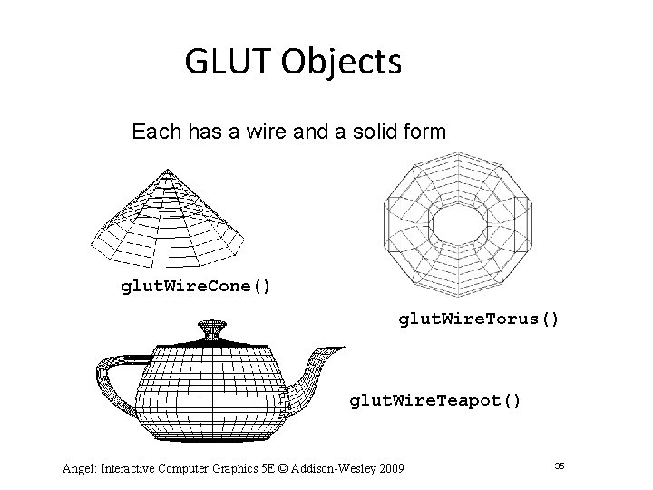
GLUT Objects Each has a wire and a solid form glut. Wire. Cone() glut. Wire. Torus() glut. Wire. Teapot() Angel: Interactive Computer Graphics 5 E © Addison-Wesley 2009 35

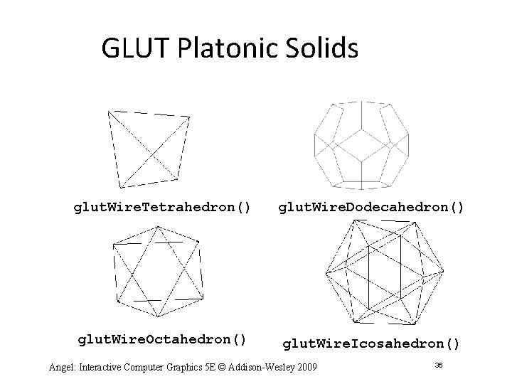
GLUT Platonic Solids glut. Wire. Tetrahedron() glut. Wire. Dodecahedron() glut. Wire. Octahedron() glut. Wire. Icosahedron() Angel: Interactive Computer Graphics 5 E © Addison-Wesley 2009 36

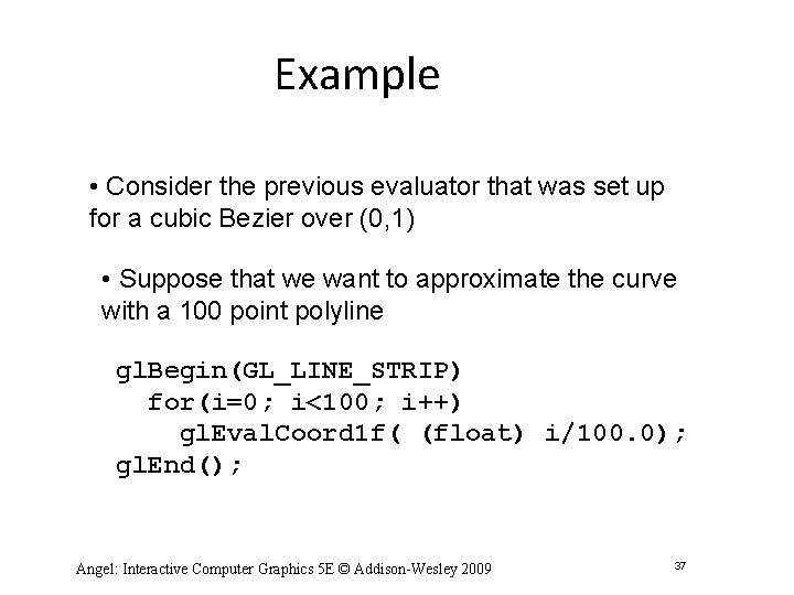
Example • Consider the previous evaluator that was set up for a cubic Bezier over (0, 1) • Suppose that we want to approximate the curve with a 100 point polyline gl. Begin(GL_LINE_STRIP) for(i=0; i<100; i++) gl. Eval. Coord 1 f( (float) i/100. 0); gl. End(); Angel: Interactive Computer Graphics 5 E © Addison-Wesley 2009 37

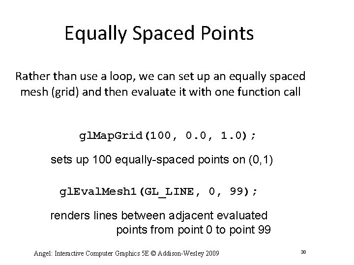
Equally Spaced Points Rather than use a loop, we can set up an equally spaced mesh (grid) and then evaluate it with one function call gl. Map. Grid(100, 0. 0, 1. 0); sets up 100 equally-spaced points on (0, 1) gl. Eval. Mesh 1(GL_LINE, 0, 99); renders lines between adjacent evaluated points from point 0 to point 99 Angel: Interactive Computer Graphics 5 E © Addison-Wesley 2009 38

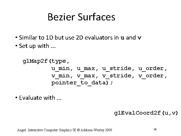
Bezier Surfaces • Similar to 1 D but use 2 D evaluators in u and v • Set up with. . . gl. Map 2 f(type, u_min, u_max, u_stride, u_order, v_min, v_max, v_stride, v_order, pointer_to_data); • Evaluate with. . . gl. Eval. Coord 2 f(u, v) Angel: Interactive Computer Graphics 5 E © Addison-Wesley 2009 39

Example bicubic patch over (0, 1) x (0, 1) point data[4][4]={………}; gl. Map 2 f(GL_MAP_VERTEX_3, 0. 0, 1. 0, 3, 4, 0. 0, 12, 4, data); Note that in v direction data points are separated by 12 floats since data array is stored by rows Angel: Interactive Computer Graphics 5 E © Addison-Wesley 2009 40

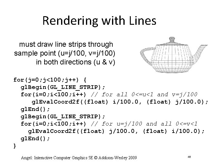
Rendering with Lines must draw line strips through sample point (u=j/100, v=j/100) in both directions (u & v) for(j=0; j<100; j++) { gl. Begin(GL_LINE_STRIP); for(i=0; i<100; i++) // for all 0<=u<1 and v=j/100 gl. Eval. Coord 2 f((float) i/100. 0, (float) j/100. 0); gl. End(); gl. Begin(GL_LINE_STRIP); for(i=0; i<100; i++) // for u=j/100 and all 0<=v<1 gl. Eval. Coord 2 f((float) j/100. 0, (float) i/100. 0); gl. End(); } Angel: Interactive Computer Graphics 5 E © Addison-Wesley 2009 41

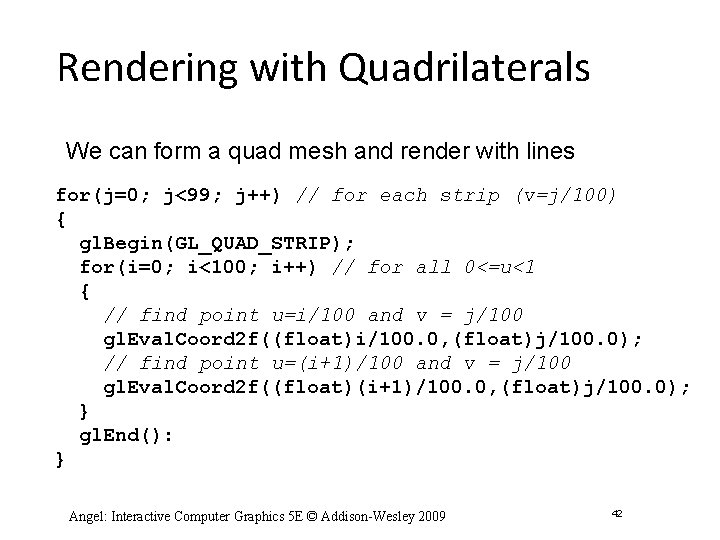
Rendering with Quadrilaterals We can form a quad mesh and render with lines for(j=0; j<99; j++) // for each strip (v=j/100) { gl. Begin(GL_QUAD_STRIP); for(i=0; i<100; i++) // for all 0<=u<1 { // find point u=i/100 and v = j/100 gl. Eval. Coord 2 f((float)i/100. 0, (float)j/100. 0); // find point u=(i+1)/100 and v = j/100 gl. Eval. Coord 2 f((float)(i+1)/100. 0, (float)j/100. 0); } gl. End(): } Angel: Interactive Computer Graphics 5 E © Addison-Wesley 2009 42

Uniform Meshes • We can form a 2 D mesh (grid) in a similar manner to 1 D for uniform spacing gl. Map. Grid 2(u_num, u_min, u_max, v_num, v_min, v_max); • Can evaluate as before with lines or if we want filled polygons. . . gl. Eval. Mesh 2(GL_FILL, u_start, u_num, v_start, v_num); Angel: Interactive Computer Graphics 5 E © Addison-Wesley 2009 43

Rendering with Lighting • If we use filled polygons, we have to shade or we will see solid color uniform rendering • Can specify lights and materials but we need normals –Let Open. GL find them gl. Enable(GL_AUTO_NORMAL); Angel: Interactive Computer Graphics 5 E © Addison-Wesley 2009 44

NURBS • Open. GL supports NURBS surfaces through the GLU library • Why GLU? –Can use evaluators in 4 D with standard Open. GL library –However, there are many complexities with NURBS that need a lot of code –There are five NURBS surface functions plus functions for trimming curves that can remove pieces of a NURBS surface Angel: Interactive Computer Graphics 5 E © Addison-Wesley 2009 45

Quadrics • Quadrics are in both the GLU and GLUT libraries –Both use polygonal approximations where the application specifies the resolution –Sphere: lines of longitude and lattitude • GLU: disks, cylinders, spheres –Can apply transformations to scale, orient, and position • GLUT: Platonic solids, torus, Utah teapot, cone Angel: Interactive Computer Graphics 5 E © Addison-Wesley 2009 46