Parameterization of surface fluxes Outline Surface layer formulation

Mixing across steep gradients Stable BL Dry mixed layer Cloudy BL Surface flux parametrization

Why is the finite difference formulation in the surface layer different from the other

Log-profiles are directly related to neutral transfer laws Lowest model level U 1, V

Low wind speeds and the limit of free convection At zero wind speed, coupling

Transfer coefficients Surface fluxes can be written explicitly as: Lowest model level U 1,

Numerical procedure: The Richardson number The expressions for surface fluxes are implicit i. e

Surface fluxes: Summary • MO-similarity provides solid basis for parametrization of surface fluxes •

Parameterization of surface fluxes: Outline • Surface layer formulation according to Monin Obukhov (MO)

Surface roughness length (definition) Example for wind: • Surface roughness length is defined on

Roughness lengths over the ocean Roughness lengths are determined by molecular diffusion and ocean

Sensitivity to changes in surface drag over ocean CM+10% CM-10% Extremely sensitive to small

Roughness length over land Geographical fields based on land use tables: Llanthony valley, S.

Longstanding near-surface wind (short-range) forecast errors 10 m wind speed bias/st dev - Europe

Derivation of a new roughness length table The 10 m winds are mainly controlled

Derivation of a new roughness length table Forecast 10 m winds error compared to

Impact on 10 m wind speed in short range forecasts OLD FC - OBS

Subgrid drag (stress) mechanisms in the ECMWF model Scales smaller than 5 km Scales

An illustration of the surface stress from the different schemes (u-component) u-component TURB stress

WGNE Drag project – comparison of surface stress PBL over water PBL+SGO over land

Changing the TOFD and low level blocking strength impacts the forecast from the very

Impact on medium range forecasts Change in RMSE Z 500 h. Pa H-TOFD H-BLOCK

Thank you training course: boundary layer; surface layer

Slides: 27

Download presentation

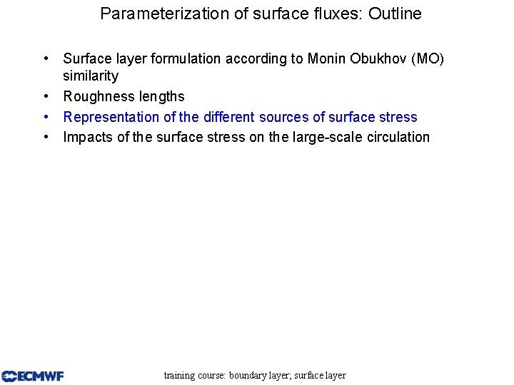
Parameterization of surface fluxes: Outline • • Surface layer formulation according to Monin Obukhov (MO) similarity Roughness lengths Representation of the different sources of surface stress Impacts of the surface stress on the large-scale circulation training course: boundary layer; surface layer

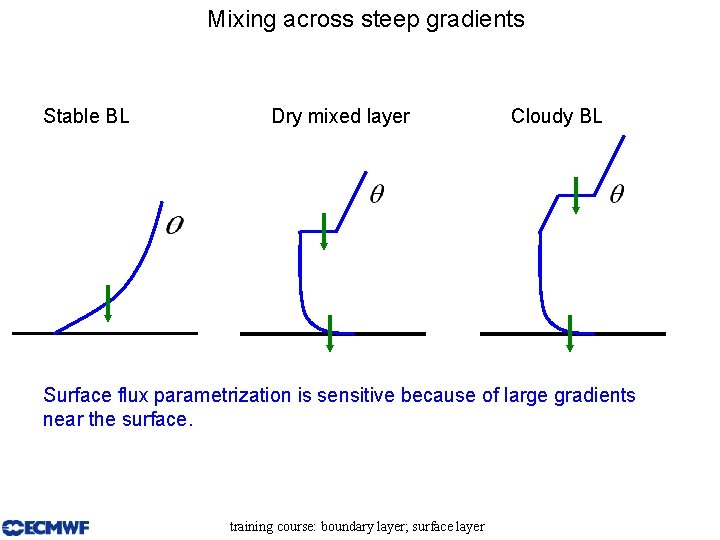
Mixing across steep gradients Stable BL Dry mixed layer Cloudy BL Surface flux parametrization is sensitive because of large gradients near the surface. training course: boundary layer; surface layer

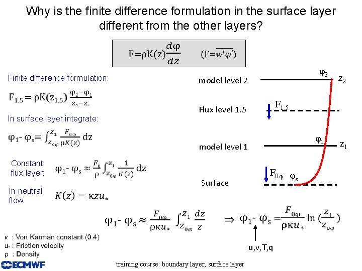
Why is the finite difference formulation in the surface layer different from the other layers? Finite difference formulation: model level 2 Flux level 1. 5 In surface layer integrate: φ2 F 1. 5 φ1 model level 1 Constant flux layer: In neutral flow: F 0φ φ s Surface u, v, T, q training course: boundary layer; surface layer z 2 z 1

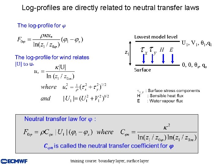
Log-profiles are directly related to neutral transfer laws Lowest model level U 1, V 1, θ 1, q 1 z 1 Surface training course: boundary layer; surface layer 0, 0, θs, qs

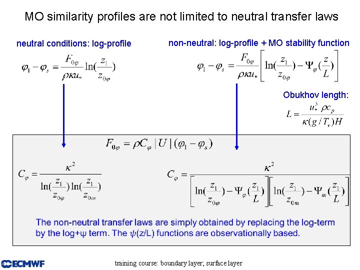
MO similarity profiles are not limited to neutral transfer laws neutral conditions: log-profile non-neutral: log-profile + MO stability function Obukhov length: training course: boundary layer; surface layer

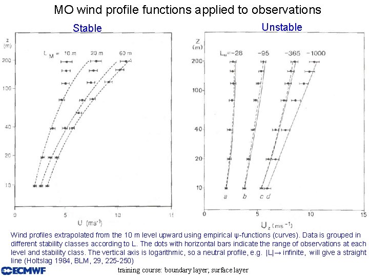
MO wind profile functions applied to observations Stable Unstable Wind profiles extrapolated from the 10 m level upward using empirical ψ-functions (curves). Data is grouped in different stability classes according to L. The dots with horizontal bars indicate the range of observations at each level and stability class. The vertical axis is logarithmic, so a neutral profile, e. g. |L|→ infinite, will give a straight line (Holtslag 1984, BLM, 29, 225 -250) training course: boundary layer; surface layer

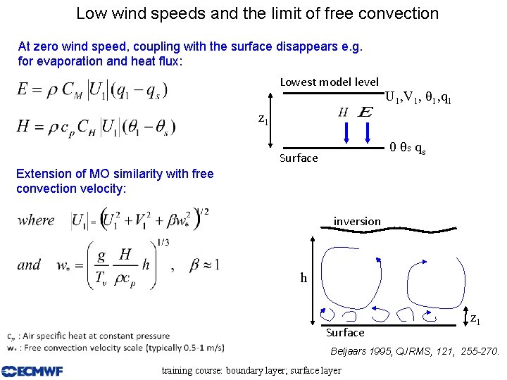
Low wind speeds and the limit of free convection At zero wind speed, coupling with the surface disappears e. g. for evaporation and heat flux: Lowest model level U 1, V 1, θ 1, q 1 z 1 0 θs qs Surface Extension of MO similarity with free convection velocity: inversion h Surface z 1 Beljaars 1995, QJRMS, 121, 255 -270. training course: boundary layer; surface layer

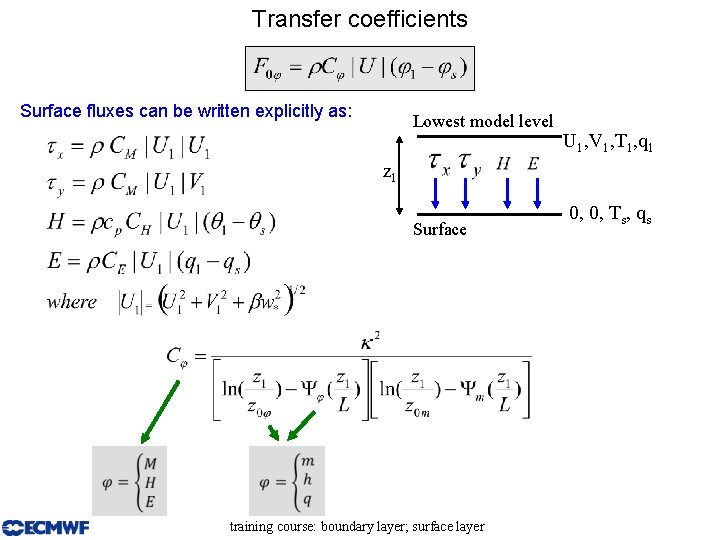
Transfer coefficients Surface fluxes can be written explicitly as: Lowest model level U 1, V 1, T 1, q 1 z 1 Surface training course: boundary layer; surface layer 0, 0, Ts, qs

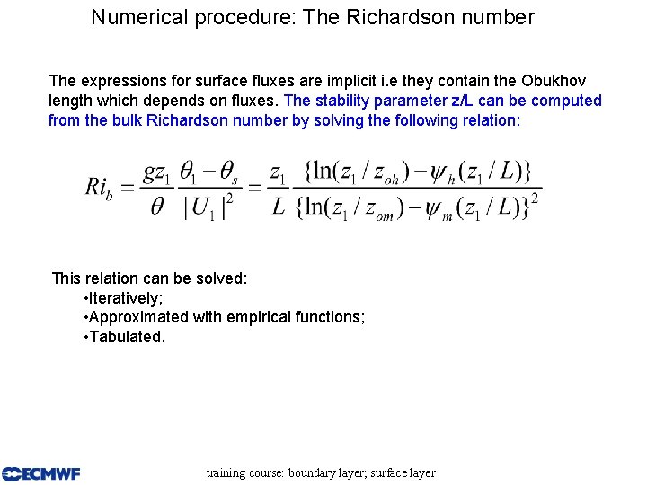
Numerical procedure: The Richardson number The expressions for surface fluxes are implicit i. e they contain the Obukhov length which depends on fluxes. The stability parameter z/L can be computed from the bulk Richardson number by solving the following relation: This relation can be solved: • Iteratively; • Approximated with empirical functions; • Tabulated. training course: boundary layer; surface layer

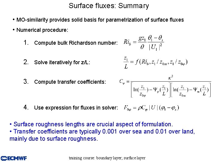
Surface fluxes: Summary • MO-similarity provides solid basis for parametrization of surface fluxes • Numerical procedure: 1. Compute bulk Richardson number: 2. Solve iteratively for z/L: 3. Compute transfer coefficients: 4. Use expression for fluxes in solver: • Surface roughness lengths are crucial aspect of formulation. • Transfer coefficients are typically 0. 001 over sea and 0. 01 over land, mainly due to surface roughness. training course: boundary layer; surface layer

Parameterization of surface fluxes: Outline • Surface layer formulation according to Monin Obukhov (MO) similarity • Roughness lengths • Representation of the different sources of surface stress • Impacts of the surface stress on the large-scale circulation training course: boundary layer; surface layer

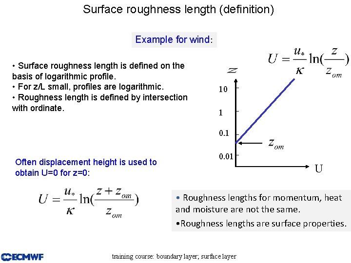
Surface roughness length (definition) Example for wind: • Surface roughness length is defined on the basis of logarithmic profile. • For z/L small, profiles are logarithmic. • Roughness length is defined by intersection with ordinate. 10 1 0. 1 Often displacement height is used to obtain U=0 for z=0: 0. 01 U • Roughness lengths for momentum, heat and moisture are not the same. • Roughness lengths are surface properties. training course: boundary layer; surface layer

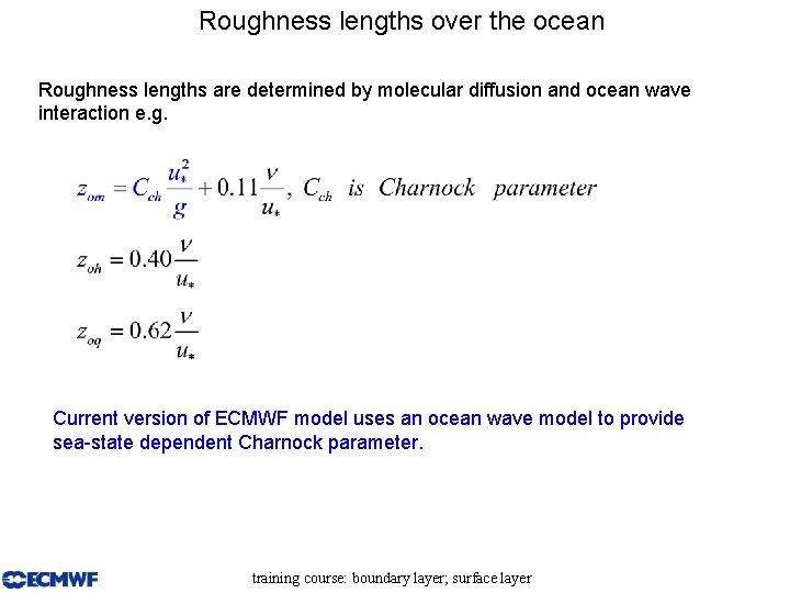
Roughness lengths over the ocean Roughness lengths are determined by molecular diffusion and ocean wave interaction e. g. Current version of ECMWF model uses an ocean wave model to provide sea-state dependent Charnock parameter. training course: boundary layer; surface layer

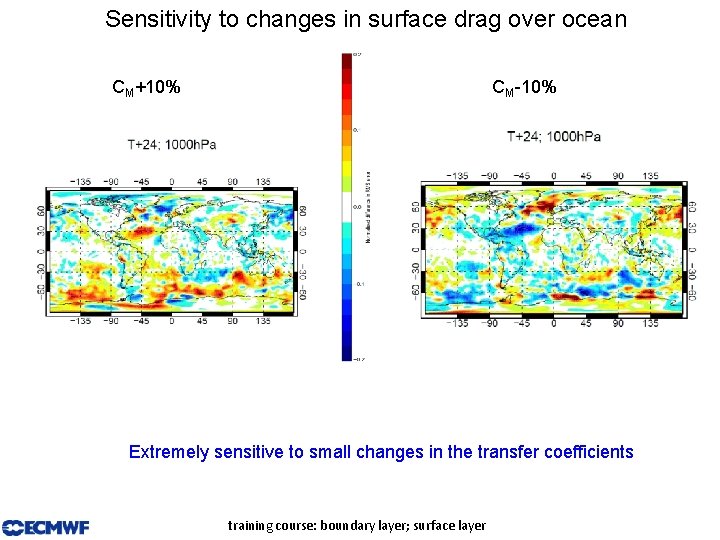
Sensitivity to changes in surface drag over ocean CM+10% CM-10% Extremely sensitive to small changes in the transfer coefficients training course: boundary layer; surface layer

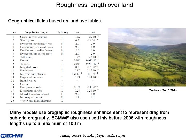
Roughness length over land Geographical fields based on land use tables: Llanthony valley, S. Wales Many models use orographic roughness enhancement to represent drag from sub-grid orography. ECMWF also used this before 2006 with roughness lengths up to a maximum of 100 m. training course: boundary layer; surface layer

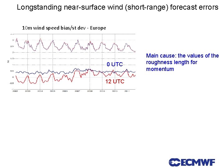
Longstanding near-surface wind (short-range) forecast errors 10 m wind speed bias/st dev - Europe 0 UTC 12 UTC Seminar MPI, 27 th of October 2014 Main cause: the values of the roughness length for momentum

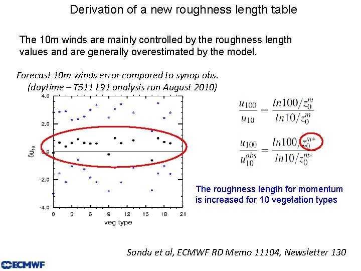
Derivation of a new roughness length table The 10 m winds are mainly controlled by the roughness length values and are generally overestimated by the model. Forecast 10 m winds error compared to synop obs. (daytime – T 511 L 91 analysis run August 2010) The roughness length for momentum is increased for 10 vegetation types Sandu et al, ECMWF RD Memo 11104, Newsletter 130

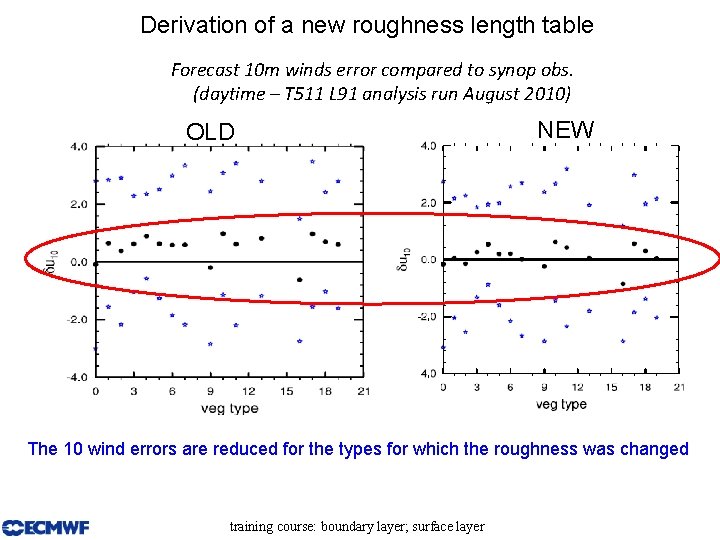
Derivation of a new roughness length table Forecast 10 m winds error compared to synop obs. (daytime – T 511 L 91 analysis run August 2010) OLD NEW The 10 wind errors are reduced for the types for which the roughness was changed training course: boundary layer; surface layer

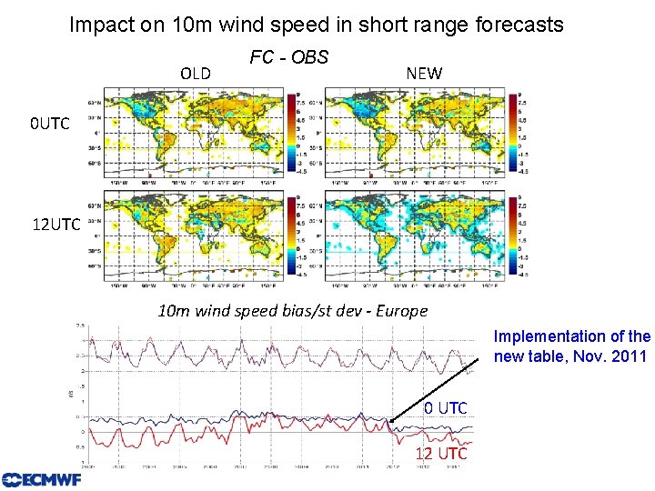
Impact on 10 m wind speed in short range forecasts OLD FC - OBS NEW 0 UTC 12 UTC 10 m wind speed bias/st dev - Europe Implementation of the new table, Nov. 2011 0 UTC 12 UTC

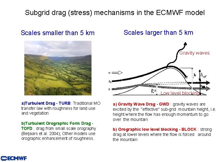
Subgrid drag (stress) mechanisms in the ECMWF model Scales smaller than 5 km Scales larger than 5 km Gravity waves h zblk Low level blocking a)Turbulent Drag - TURB: Traditional MO transfer law with roughness for land use and vegetation b)Turbulent Orographic Form Drag TOFD : drag from small scale orography (Beljaars et al. 2004); Other models use orographic enhancement of roughness. a) Gravity Wave Drag - GWD : gravity waves are excited by the “effective” sub-grid mountain height, i. e. height where the flow has enough momentum to go over the mountain b) Orographic low level blocking - BLOCK : strong drag at lower levels where the flow is forced around the mountain

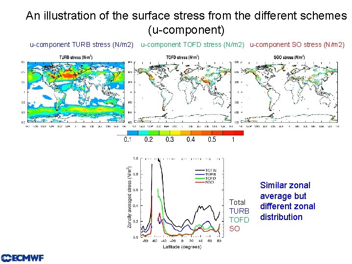
An illustration of the surface stress from the different schemes (u-component) u-component TURB stress (N/m 2) u-component TOFD stress (N/m 2) u-component SO stress (N/m 2) Total TURB TOFD SO Similar zonal average but different zonal distribution

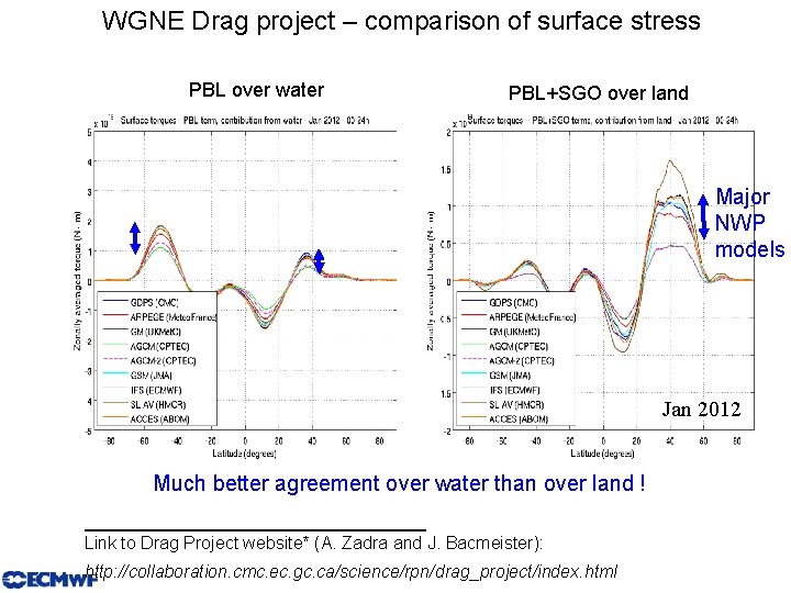
WGNE Drag project – comparison of surface stress PBL over water PBL+SGO over land Major NWP models Jan 2012 Much better agreement over water than over land ! __________________ Link to Drag Project website* (A. Zadra and J. Bacmeister): http: //collaboration. cmc. ec. gc. ca/science/rpn/drag_project/index. html

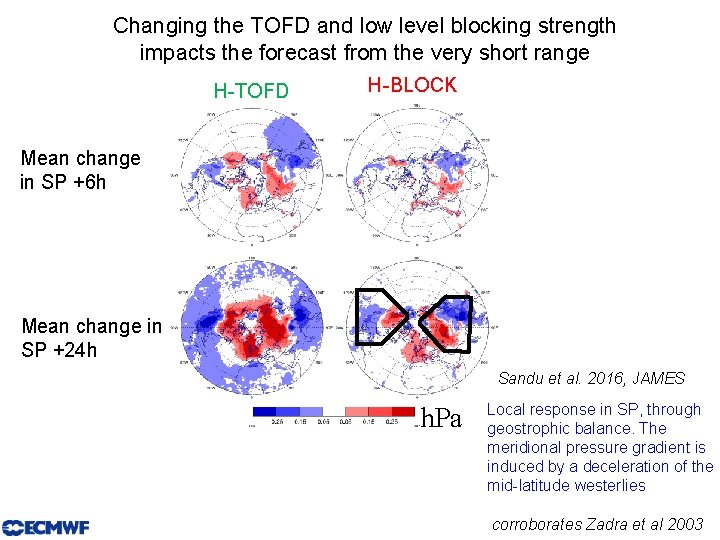
Changing the TOFD and low level blocking strength impacts the forecast from the very short range H-TOFD H-BLOCK Mean change in SP +6 h Mean change in SP +24 h Sandu et al. 2016, JAMES h. Pa Local response in SP, through geostrophic balance. The meridional pressure gradient is induced by a deceleration of the mid-latitude westerlies corroborates Zadra et al 2003

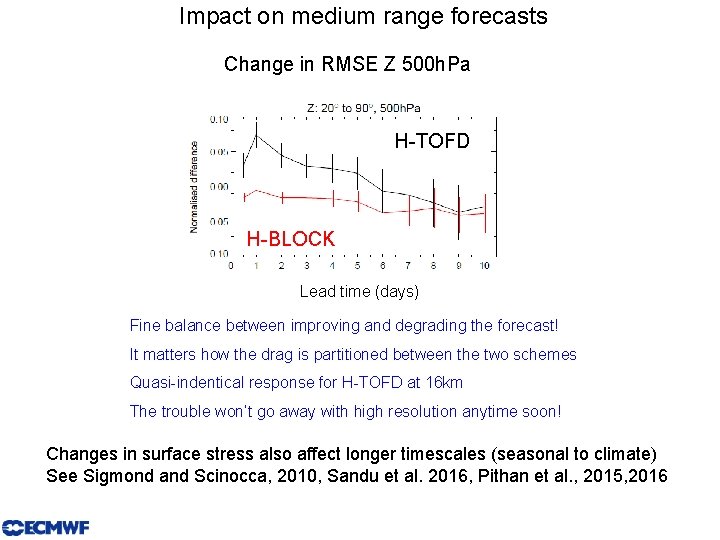
Impact on medium range forecasts Change in RMSE Z 500 h. Pa H-TOFD H-BLOCK Lead time (days) Fine balance between improving and degrading the forecast! It matters how the drag is partitioned between the two schemes Quasi-indentical response for H-TOFD at 16 km The trouble won’t go away with high resolution anytime soon! Changes in surface stress also affect longer timescales (seasonal to climate) See Sigmond and Scinocca, 2010, Sandu et al. 2016, Pithan et al. , 2015, 2016

Thank you training course: boundary layer; surface layer