Parameterization of SRF Cavity Data Filis Coba University

Parameterization of SRF Cavity Data Filis Coba, University of Central Connecticut Andrew Hutton, Jefferson Lab

Concept • The usual way of plotting SRF cavity data is a semi-log plot of the cavity Q (the cavity quality factor) versus Eacc (the accelerating gradient) • The semi-log plot is designed to focus attention on the highgradient degradation of the cavity Q, but in doing so the plot obscures the cavity response at lower gradient where the cavities are usually operated

ILC Cavity A 11

Formalism • In this presentation, the cavity performance is described by a linear plot of the surface resistance Rs in ohm versus Eacc in MV/m • The surface resistance is inversely proportional to the cavity Q (Rs = G/Q), where G is the cavity geometry factor • G is usually 250 -300Ω for electron cavities • G can be as low as 100Ω for proton cavities • The reason for focusing attention on the surface resistance is to link the cavity performance to small sample data

Surface Resistance versus Peak Magnetic Field

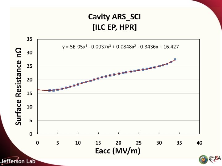
Initial curve fitting • Cavity data was exported from the JLab database, Pansophy, into an Excel spreadsheet • The cavity Q data was converted to surface resistance and the data plotted on a linear scale • The Excel trending tool was then used to evaluate different fitting algorithms • The data could never be fitted with an exponential, logarithmic or power function • A fourth order polynomial provided an excellent fit to the data in all cases, with R 2 (the square of the Pearson product moment correlation coefficient) usually >0. 97

Observations • The fourth order polynomial fit equation is written as: Rs = AE 4 + BE 3 + CE 2 + DE + R 0 where R 0 is the zero-field surface resistance. • The data could always be described by five constants • The coefficients of E and E 3 were always negative, while the other coefficients were always positive • There a few typical features of the plots: • The curve trends upwards with increasing gradient • There is an initial decrease in the low field region • There is a “bump” in the middle field region • There is a steep rise in the high field region

Independent Features? • It is tempting to consider these features as independent, and this is how they have usually been considered. However: • The middle field bump would need three parameters to characterize it: a field value for the centre of the bump, a parameter describing the width, and a parameter describing the height. The same is true for the high field rise, while the low field decrease would need only two parameters as the feature is centred on the vertical axis • So treating the features as fully independent requires a total of eight parameters • But, it is possible to fit the data with only five parameters • The implication is that there is an inter-relationship between the features

Alternative fitting formalism • The five parameters have no apparent physical significance so an alternative formalism based on an analysis of the shape of the features was developed • The first step was to fit the general upward trend of the curve with a linear equation T + S. E • S is the slope of the line and • T is the intercept on the R axis (E = 0) • S and T should be independent of high- field data • On occasion, the highest gradients cannot be reached due to lack of RF power • Since the lowest value of the surface resistance is obtained with the best surfaces, the straight line should be on the low side of the curve

Linear Fit • The only line that can drawn that meets these criteria touches the curve tangentially at two points • U, RU, at the onset of the middle field regime • V, RV, at the onset of the high field regime • The constants S and T can be derived easily from these two points: S = (RV – RU)/(V –U) T = RU – S. U

Fitting Higher Orders • Subtract the straight line from the fourth order polynomial fit • The resulting curve has zero surface resistance at two points where Eacc = U and V • The slope of the curve at these two points is also zero • Elsewhere, the curve is positive definite because of the way the straight line was selected • The goal is to find an expression that meets these criteria using only three variables, one of which must be a vertical scale factor • The only expression that meets all of these criteria is of form (scale factor). (1 -E/U)2. (1 -E/V)2 • The scale factor is determined by calculating the surface resistance R 0 at E = 0 • The scale factor turns out to be (R 0 – T)

Final Equation Rs = T + S × E + {Ro– T} × {1– (E/U)}2 × {1– (E/V)}2 where • Rs is the surface resistance at Eacc = E • S is the slope of the straight line • T is the intercept of the straight line on the R axis • R 0 is the value of the surface resistance at Eacc = 0 • U and V are the values of E where the straight line touches the fourth order polynomial fit to the data

Fitting S and T R 0 e Slop S V T U

Relationship between Equations • The data has been fitted by two equations, a fourth order polynomial and a more complex equation • The two can be inter-related by expanding and comparing the coefficients of like terms. After some straightforward (but messy) algebra, the following results are obtained: S = – D – B(C/A – B 2/4 A 2)/2 T = R 0 – A(C/A – B 2/4 A 2)/2}2 U = {–B – (3 B 2 – 8 AC)½}/4 A 2 V = {–B + (3 B 2 – 8 AC)½}/4 A 2

Change of Independent variable • This formalism can be extended to other independent variables • E. g. peak electric field Epeak and the peak magnetic field Hpeak • The ratio of these parameters to the accelerating gradient Eacc is known for each cavity shape, so converting the horizontal axis is straightforward. • The fitting parameters R 0 and T remain unchanged in this transformation, while the other three parameters are scaled by the ratio of Epeak/Eacc or Hpeak/Eacc • The change in independent variable can provide additional information by comparing cavities of different shapes • When the ratios of Epeak/Eacc and Hpeak/Eacc are different, comparing data from different cavity shapes may help define the driving physical phenomena

Evaluation of ILC Cavities • 25 ILC 9 -cell cavity measurement sets have been fitted with this technique • 18 from ACCEL/RI on 9 different cavities • 4 from AES on 4 different cavities • 2 from JLab on 1 cavity • 1 from PKU • The five fitting parameters and Emax are tabulated in the next slide • Cavities with highest Emax are on top

Summary • A parameterization of the SRF data has been obtained which fits all of the ILC data • It can be used to provide a way to categorize the data • Previous data sets only give the Q at Emax • For cavities destined for CW use, this is not sufficient • The parameterization may or may not have any fundamental significance