Parameterization of continental surfaces in coupled Earth System

Parameterization of continental surfaces in coupled Earth System Modelling: part III How surface processes influence Earth System predictability? Gianpaolo Balsamo Coupling Processes Team, Earth System Model Section gianpaolo. balsamo@ecmwf. int © ECMWF March 6, 2021

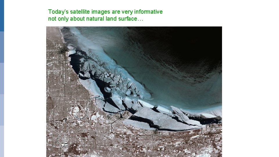
Today’s satellite images are very informative not only about natural land surface…

Context • Why Numerical Weather Prediction had to embrace Earth System Modelling? – It is much nicer and represent nature better? Do we gain? • Biosphere, Hydrosphere, Cryosphere, and Atmosphere: Do they all matter the same? – Can we attempt a quantitative evaluation? What are the caveats? • Diurnal and Seasonal amplitude improvements – How much are they drivers to accurate predictions? • What else is in the “hat” and where do we need (r)evolutionary ideas? – Bridging gaps between modelling communities. – Bringing new EO data to guide model development • Roadmap to Global Environmental Monitoring and Prediction – If we can imagine it, probably we can do it? EUROPEAN CENTRE FOR MEDIUM-RANGE WEATHER FORECASTS October 29, 2014 3

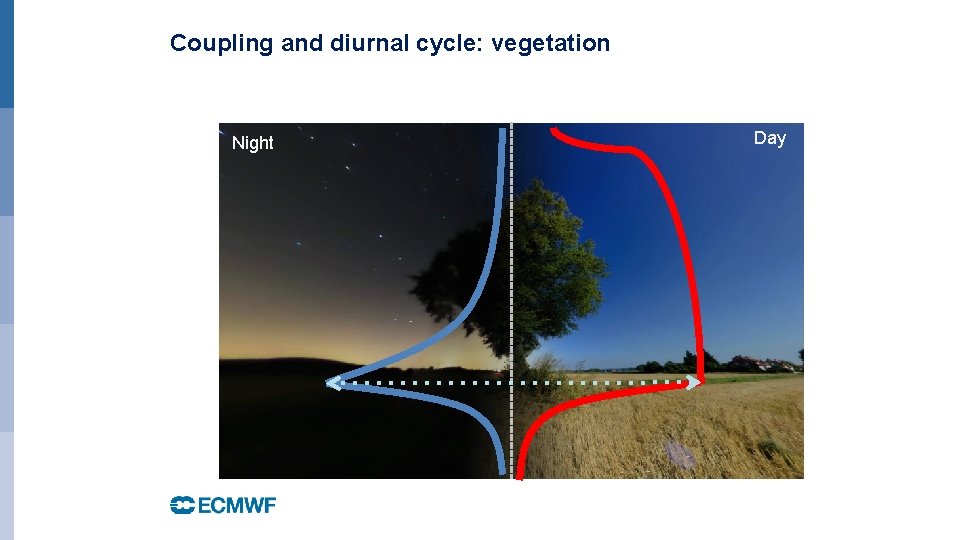
Coupling and diurnal cycle: vegetation Night Day

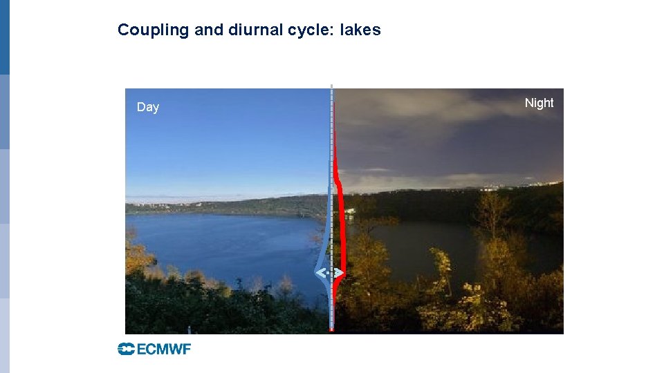
Coupling and diurnal cycle: lakes Day Night

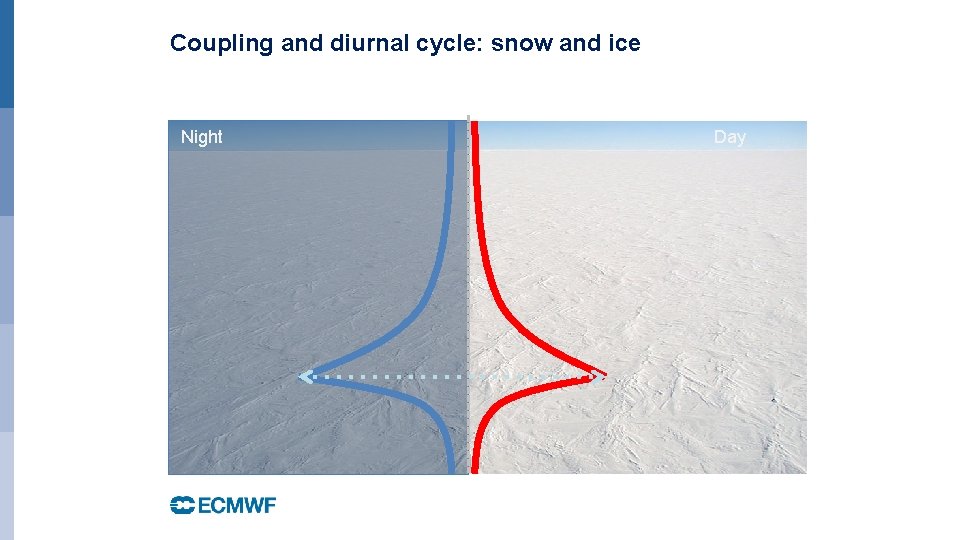
Coupling and diurnal cycle: snow and ice Night Day

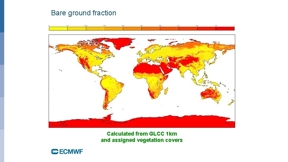
Bare ground fraction Calculated from GLCC 1 km and assigned vegetation covers

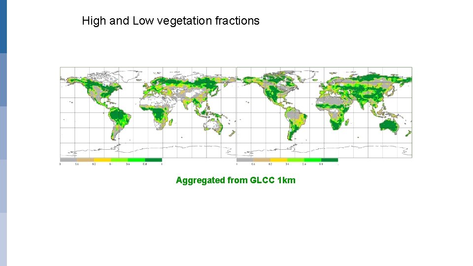
High and Low vegetation fractions Aggregated from GLCC 1 km

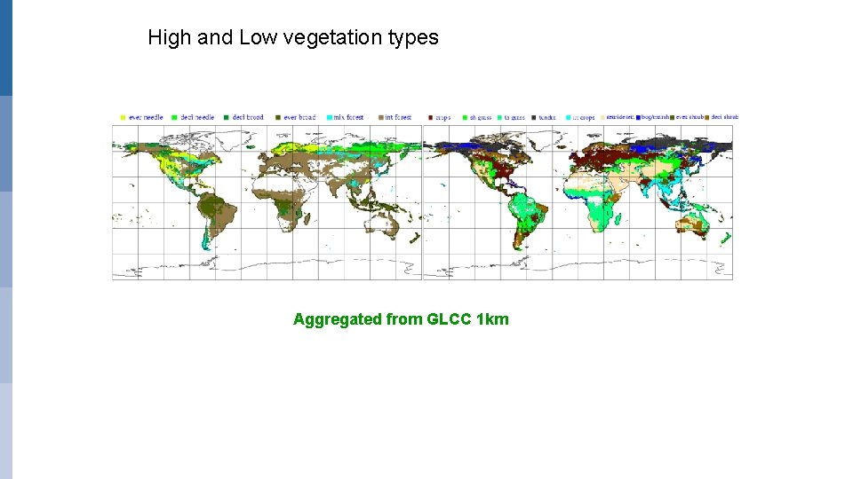
High and Low vegetation types Aggregated from GLCC 1 km

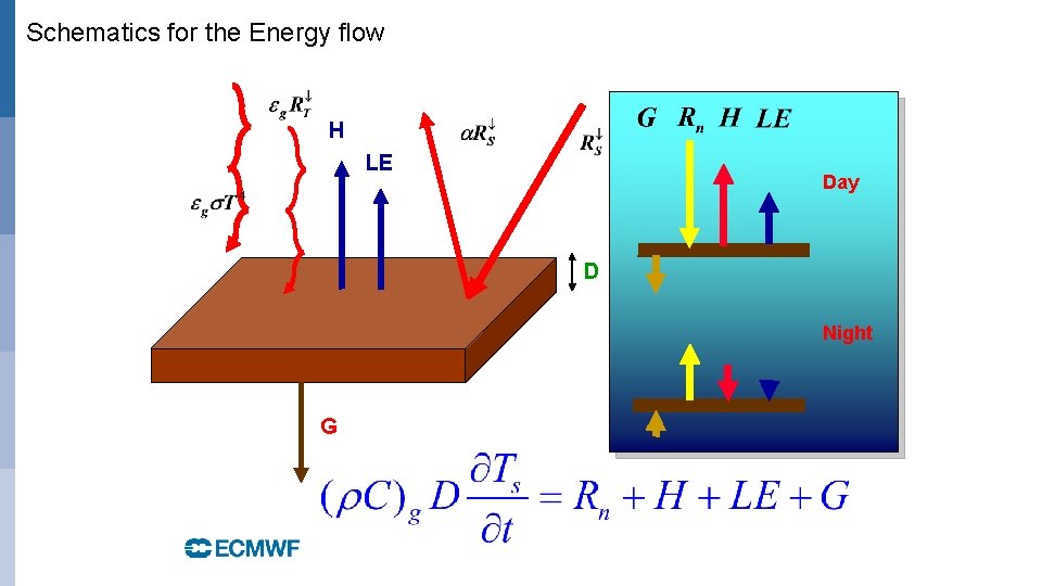
Schematics for the Energy flow H LE Day D Night G

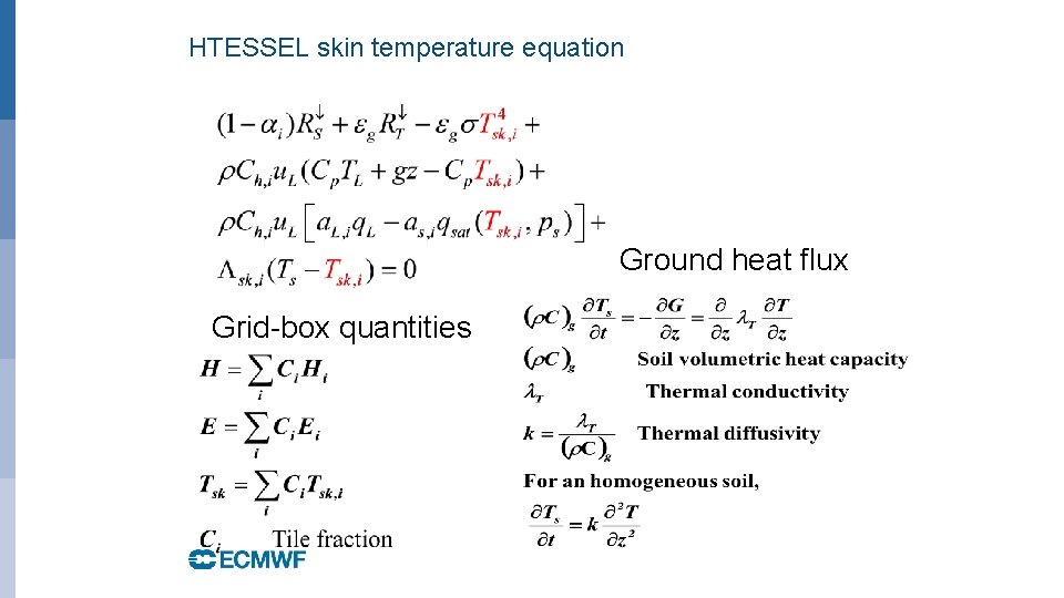
HTESSEL skin temperature equation Ground heat flux • Grid-box quantities

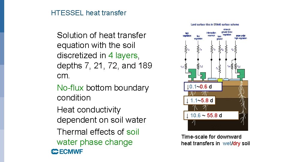
HTESSEL heat transfer • Solution of heat transfer equation with the soil discretized in 4 layers, depths 7, 21, 72, and 189 cm. • No-flux bottom boundary condition • Heat conductivity dependent on soil water • Thermal effects of soil water phase change ↓ 0. 1~0. 6 d ↓ 1. 1~5. 8 d ↓ 10. 6 ~ 55. 8 d Time-scale for downward heat transfers in wet/dry soil

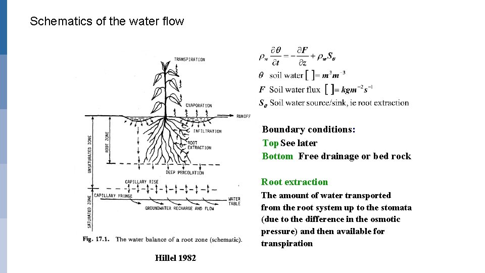
Schematics of the water flow Boundary conditions: Top. See later Bottom Free drainage or bed rock Root extraction The amount of water transported from the root system up to the stomata (due to the difference in the osmotic pressure) and then available for transpiration Hillel 1982

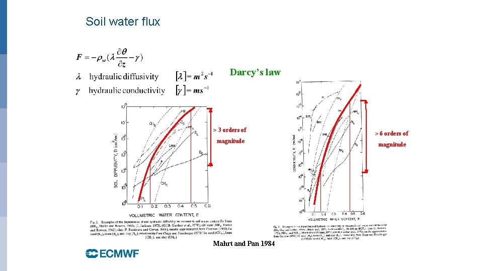
Soil water flux Darcy’s law > 3 orders of magnitude Mahrt and Pan 1984 > 6 orders of magnitude

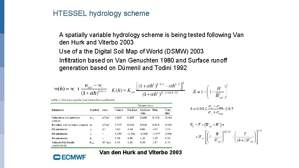
HTESSEL hydrology scheme • A spatially variable hydrology scheme is being tested following Van den Hurk and Viterbo 2003 • Use of a the Digital Soil Map of World (DSMW) 2003 • Infiltration based on Van Genuchten 1980 and Surface runoff generation based on Dümenil and Todini 1992 Van den Hurk and Viterbo 2003

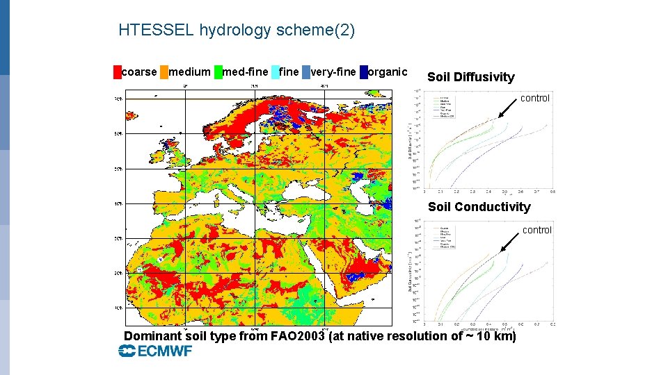
HTESSEL hydrology scheme(2) █coarse █medium █med-fine █very-fine █organic Soil Diffusivity control Soil Conductivity control Dominant soil type from FAO 2003 (at native resolution of ~ 10 km)

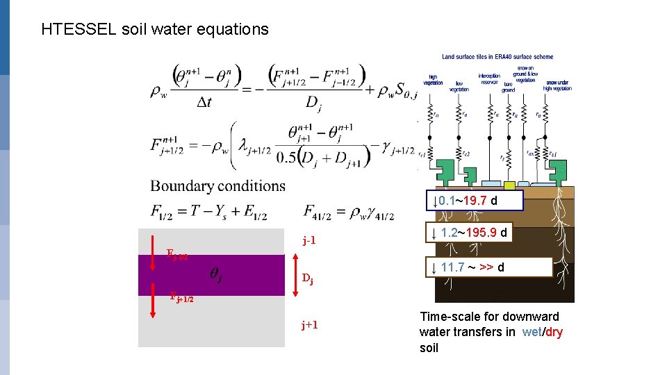
HTESSEL soil water equations ↓ 0. 1~19. 7 d j-1 Fj-1/2 Dj ↓ 1. 2~195. 9 d ↓ 11. 7 ~ >> d Fj+1/2 j+1 Time-scale for downward water transfers in wet/dry soil

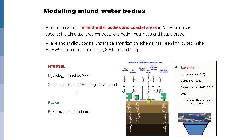
Modelling inland water bodies A representation of inland water bodies and coastal areas in NWP models is essential to simulate large contrasts of albedo, roughness and heat storage A lake and shallow coastal waters parametrization scheme has been introduced in the ECMWF Integrated Forecasting System combining HTESSEL Lake tile Hydrology - Tiled ECMWF Mironov et al (2010), Dutra et al. (2010), Scheme for Surface Exchanges over Land + FLake Fresh water Lake scheme Balsamo et al. (2010, 2012, 2013) Extra tile (9) to account for sub-grid lakes

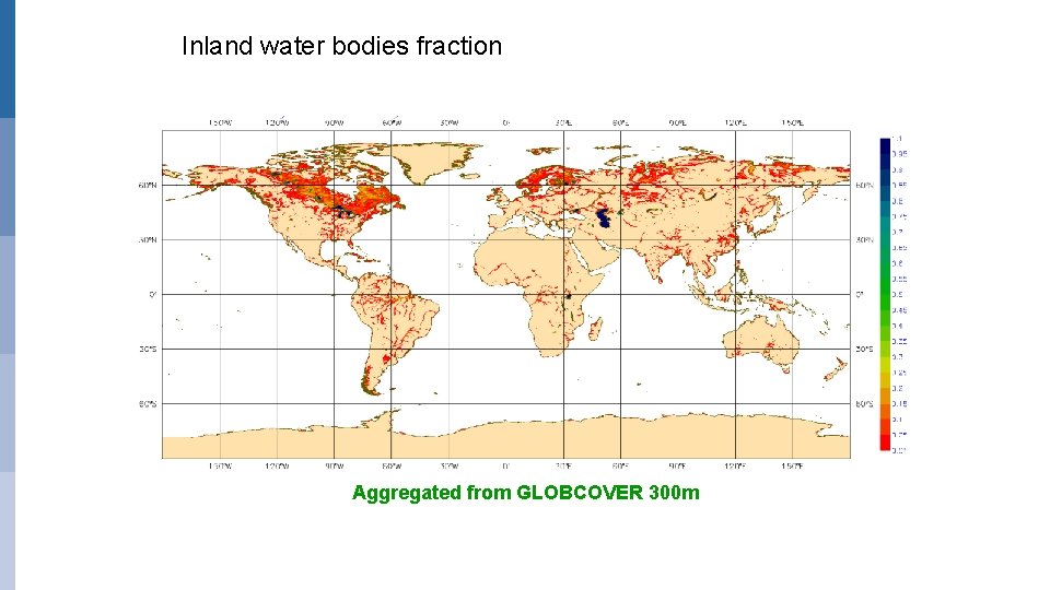
Inland water bodies fraction Aggregated from GLOBCOVER 300 m

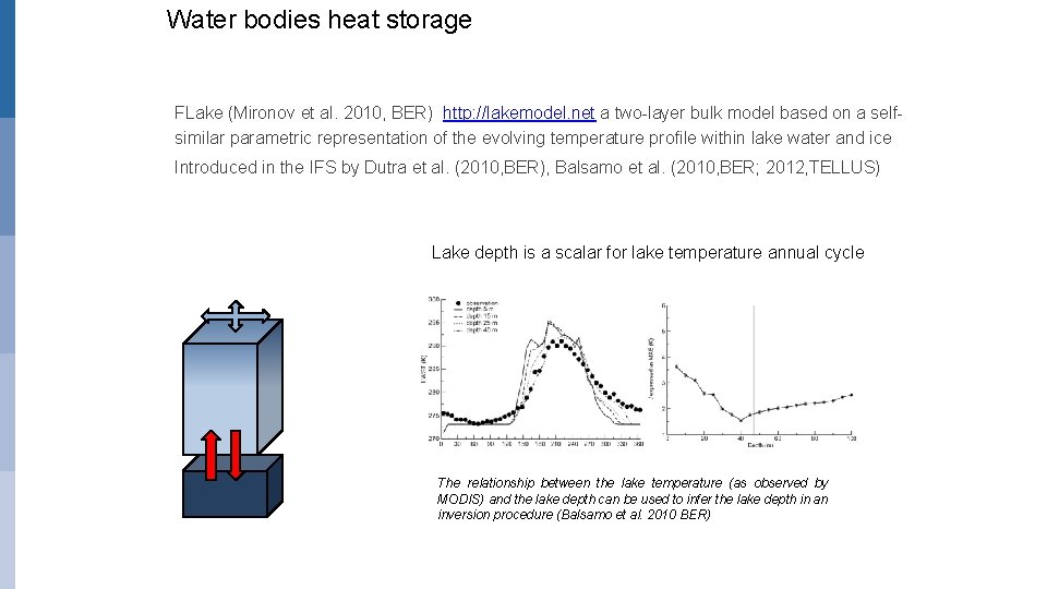
Water bodies heat storage • All inland water bodies are important energy storage drastically changing sensible heat flux • FLake (Mironov et al. 2010, BER) http: //lakemodel. net a two-layer bulk model based on a selfsimilar parametric representation of the evolving temperature profile within lake water and ice • Introduced in the IFS by Dutra et al. (2010, BER), Balsamo et al. (2010, BER; 2012, TELLUS) Lake depth is a scalar for lake temperature annual cycle The relationship between the lake temperature (as observed by MODIS) and the lake depth can be used to infer the lake depth in an inversion procedure (Balsamo et al. 2010 BER)

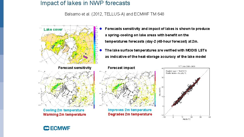
Impact of lakes in NWP forecasts Balsamo et al. (2012, TELLUS-A) and ECMWF TM 648 Lake cover Forecasts sensitivity and impact of lakes is shown to produce a spring-cooling on lake areas with benefit on the temperatures forecasts (day-2 (48 -hour forecast) at 2 m. The lake surface temperatures are verified with MODIS LSTs as indicative of the heat-storage accuracy of the lake model Forecast sensitivity Cooling 2 m temperature Warming 2 m temperature Forecast impact Improves 2 m temperature Degrades 2 m temperature

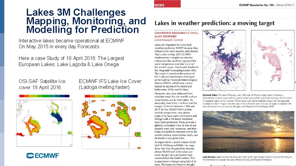
Lakes are the last newly added tile to ECMWF land surface scheme that went in operational use on the 12 th of May 2015. The importance of lakes and their temperature and ice conditions in generating clouds and storms can be appreciated in the video here: http: //time. com/9480/great-lakes-frozen-time-lapse-video/

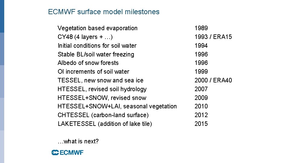
ECMWF surface model milestones • • • Vegetation based evaporation CY 48 (4 layers + …) Initial conditions for soil water Stable BL/soil water freezing Albedo of snow forests OI increments of soil water TESSEL, new snow and sea ice HTESSEL, revised soil hydrology HTESSEL+SNOW, revised snow HTESSEL+SNOW+LAI, seasonal vegetation CHTESSEL (carbon-land surface) LAKETESSEL (addition of lake tile) • …what is next? Slide 23 1989 1993 / ERA 15 1994 1996 1999 2000 / ERA 40 2007 2009 2010 2012 2015

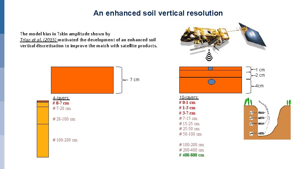
An enhanced soil vertical resolution The model bias in Tskin amplitude shown by Trigo et al. (2015) motivated the development of an enhanced soil vertical discretisation to improve the match with satellite products. 1 cm 2 cm 7 cm 4 -layers: # 0 -7 cm # 7 -28 cm # 28 -100 cm # 100 -289 cm 10 -layers: # 0 -1 cm # 1 -3 cm # 3 -7 cm # 7 -15 cm # 15 -25 cm # 25 -50 cm # 50 -100 cm # 100 -200 cm # 200 -400 cm # 400 -800 cm

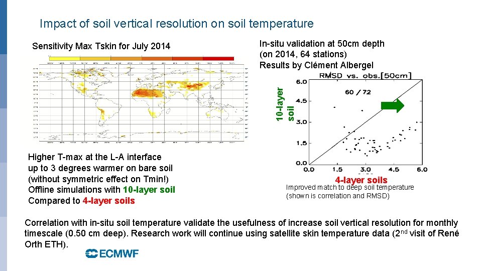
Impact of soil vertical resolution on soil temperature In-situ validation at 50 cm depth (on 2014, 64 stations) Results by Clément Albergel 10 -layer soil Sensitivity Max Tskin for July 2014 Higher T-max at the L-A interface up to 3 degrees warmer on bare soil (without symmetric effect on Tmin!) Offline simulations with 10 -layer soil Compared to 4 -layer soils Improved match to deep soil temperature (shown is correlation and RMSD) Correlation with in-situ soil temperature validate the usefulness of increase soil vertical resolution for monthly timescale (0. 50 cm deep). Research work will continue using satellite skin temperature data (2 nd visit of René Orth ETH).

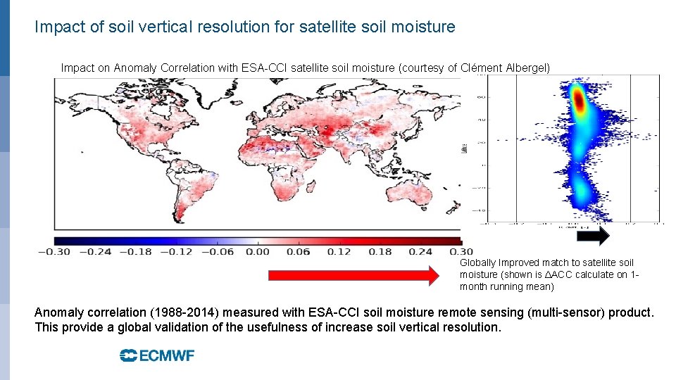
Impact of soil vertical resolution for satellite soil moisture Impact on Anomaly Correlation with ESA-CCI satellite soil moisture (courtesy of Clément Albergel) Globally Improved match to satellite soil moisture (shown is ΔACC calculate on 1 month running mean) Anomaly correlation (1988 -2014) measured with ESA-CCI soil moisture remote sensing (multi-sensor) product. This provide a global validation of the usefulness of increase soil vertical resolution.

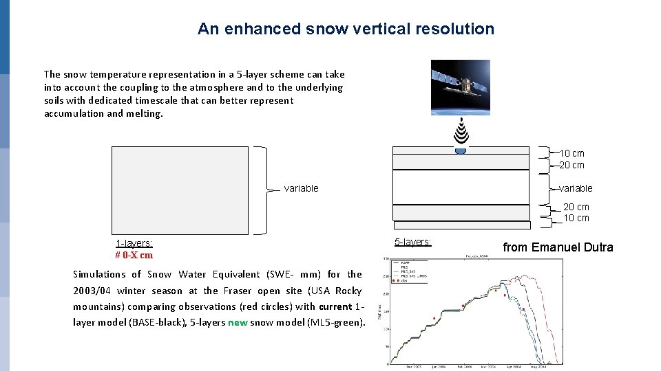
An enhanced snow vertical resolution The snow temperature representation in a 5 -layer scheme can take into account the coupling to the atmosphere and to the underlying soils with dedicated timescale that can better represent accumulation and melting. 10 cm 20 cm variable 20 cm 1 -layers: # 0 -X cm Simulations of Snow Water Equivalent (SWE- mm) for the 2003/04 winter season at the Fraser open site (USA Rocky mountains) comparing observations (red circles) with current 1 layer model (BASE-black), 5 -layers new snow model (ML 5 -green). 5 -layers: from Emanuel Dutra

Lakes 3 M Challenges Mapping, Monitoring, and Modelling for Prediction Interactive lakes became operational at ECMWF On May 2015 in every day Forecasts Here a case Study of 18 April 2016: The Largest European Lakes: Lake Lagoda & Lake Onega OSI-SAF Satellite Ice cover 18 April 2016 ECMWF IFS Lake Ice Cover (Ladoga melting faster) October 29, 2014 28

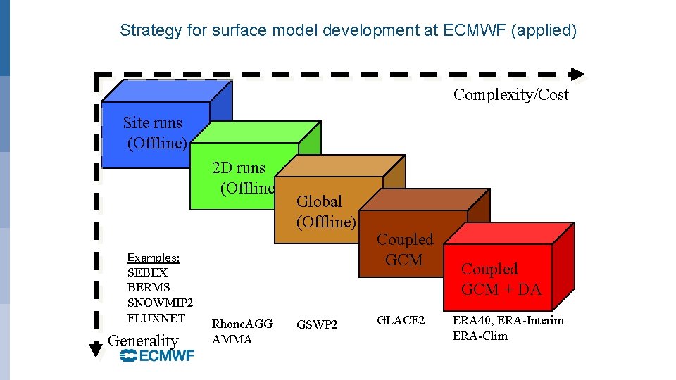
Strategy for surface model development at ECMWF (applied) Complexity/Cost Site runs (Offline) 2 D runs (Offline) Examples: SEBEX BERMS SNOWMIP 2 FLUXNET Generality Rhone. AGG AMMA Global (Offline) GSWP 2 Coupled GCM GLACE 2 Slide 29 Coupled GCM + DA ERA 40, ERA-Interim ERA-Clim

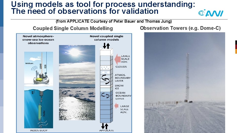
Using models as tool for process understanding: The need of observations for validation (from APPLICATE Courtesy of Peter Bauer and Thomas Jung) Coupled Single Column Modelling Observation Towers (e. g. Dome-C)

Perspectives • Efforts to improve diurnal and seasonal cycles of surface state variables has transferred into weather and climate improvements and this it will continue (doing things better may not sound attractive but it pays off!) • Surface complexity is needed and permitted by the overall skill of the atmospheric processes. • Surface representation requirements for higher resolution will not saturate at a given scale. • Earth-Observation from Satellites provide guidance for improving processes (not only useful in the data assimilation step, but also in the model development phase) and justify complexity. • In-situ data will provide guidance on process-level fidelity of a scheme. That cannot be expected at global scale and therefore in-situ data will always be a crucial part of verification. • Human influence on the surface (such as urbanization, irrigation) is yet to be represented in many models that can no longer assume natural surfaces to be static (priority not only at ECMWF). EUROPEAN CENTRE FOR MEDIUM-RANGE WEATHER FORECASTS October 29, 2014 31

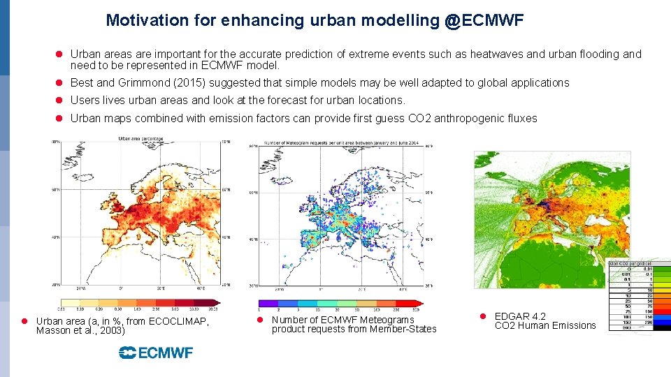
Motivation for enhancing urban modelling @ECMWF Urban areas are important for the accurate prediction of extreme events such as heatwaves and urban flooding and need to be represented in ECMWF model. Best and Grimmond (2015) suggested that simple models may be well adapted to global applications Users lives urban areas and look at the forecast for urban locations. Urban maps combined with emission factors can provide first guess CO 2 anthropogenic fluxes Urban area (a, in %, from ECOCLIMAP, Masson et al. , 2003) Number of ECMWF Meteograms product requests from Member-States EDGAR 4. 2 CO 2 Human Emissions

Closing remarks Surface-state (in the Biosphere, Cryosphere and Hydrosphere compartments) and near-surface atmospheric variables are likely to gain importance as forecasts products per-se. EUROPEAN CENTRE FOR MEDIUM-RANGE WEATHER FORECASTS 33