Parallelization of Sparse Coding Dictionary Learning University of

Parallelization of Sparse Coding & Dictionary Learning University of Colorado Denver Parallel Distributed System Fall 2016 Huynh Manh 10/3/2020 1

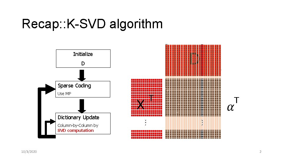
Recap: : K-SVD algorithm D Initialize D Sparse Coding Use MP X T T Dictionary Update Column-by-Column by SVD computation 10/3/2020 2

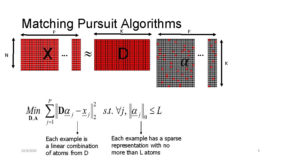
Matching Pursuit Algorithms K P X N 10/3/2020 Each example is a linear combination of atoms from D D P Each example has a sparse representation with no more than L atoms A K 3

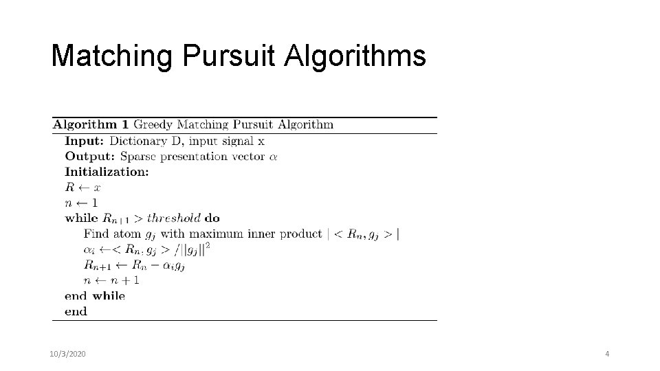
Matching Pursuit Algorithms 10/3/2020 4

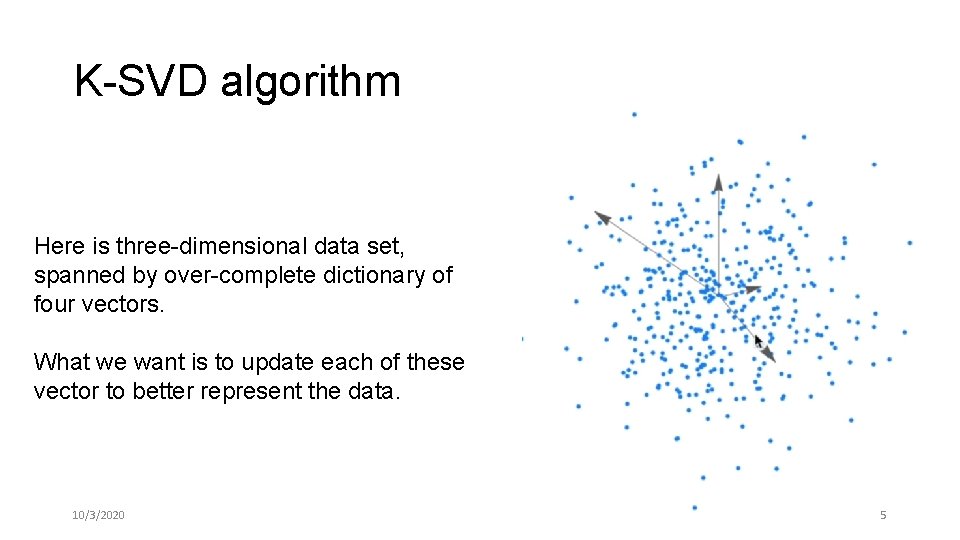
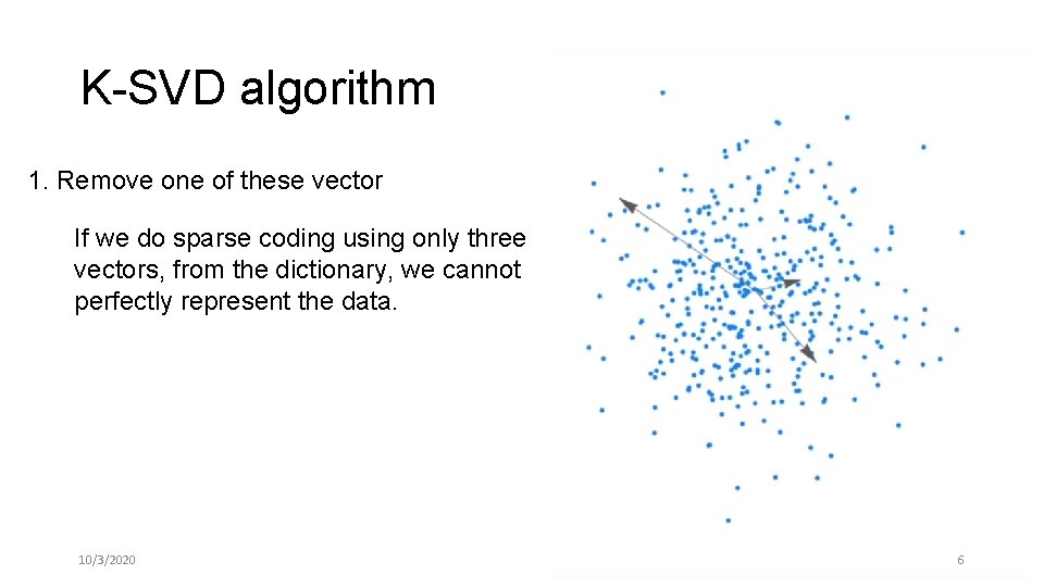
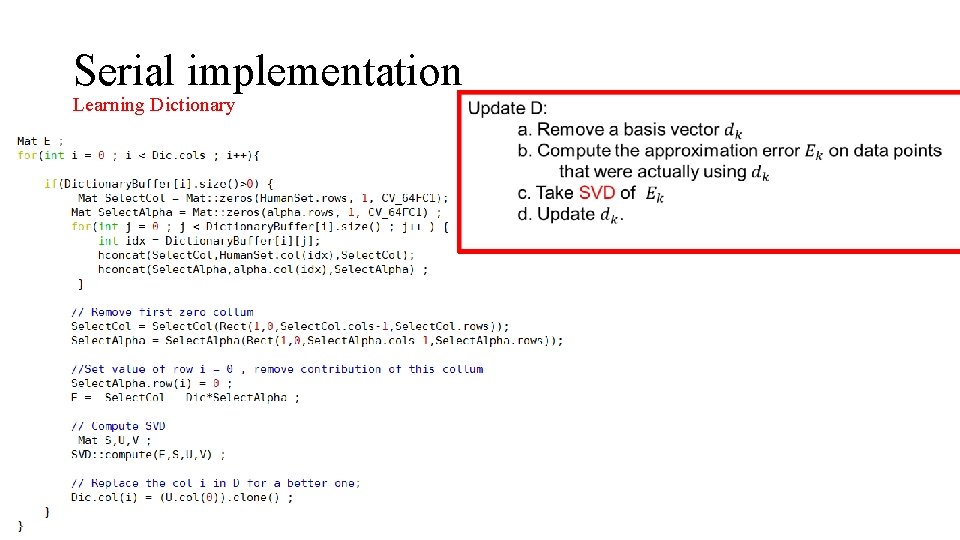
K-SVD algorithm Here is three-dimensional data set, spanned by over-complete dictionary of four vectors. What we want is to update each of these vector to better represent the data. 10/3/2020 5

K-SVD algorithm 1. Remove one of these vector If we do sparse coding using only three vectors, from the dictionary, we cannot perfectly represent the data. 10/3/2020 6

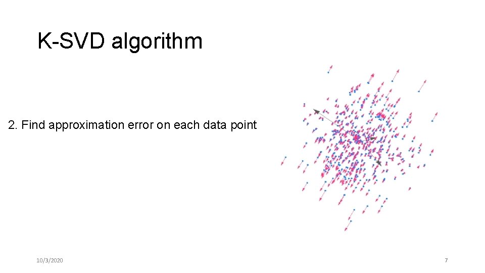
K-SVD algorithm 2. Find approximation error on each data point 10/3/2020 7

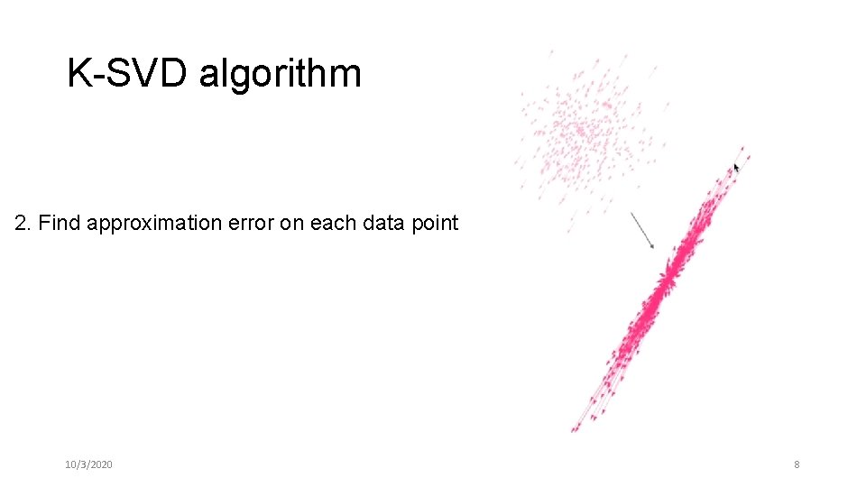
K-SVD algorithm 2. Find approximation error on each data point 10/3/2020 8

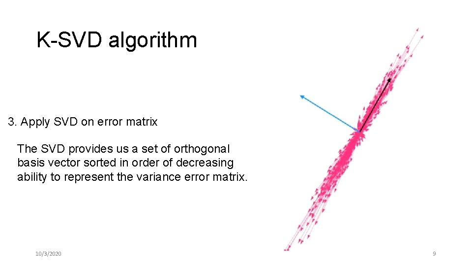
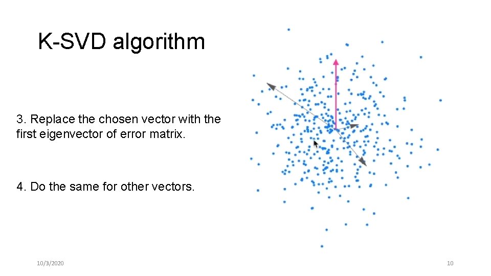
K-SVD algorithm 3. Apply SVD on error matrix The SVD provides us a set of orthogonal basis vector sorted in order of decreasing ability to represent the variance error matrix. 10/3/2020 9

K-SVD algorithm 3. Replace the chosen vector with the first eigenvector of error matrix. 4. Do the same for other vectors. 10/3/2020 10

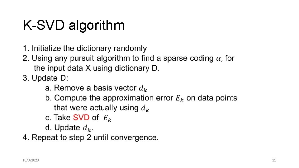
K-SVD algorithm • 10/3/2020 11

Content • Tracking framework • Feature extraction • Singular Decomposition Value (SVD) • Serial implementation. • GPU implementation and comparisons. • A summary • Next work

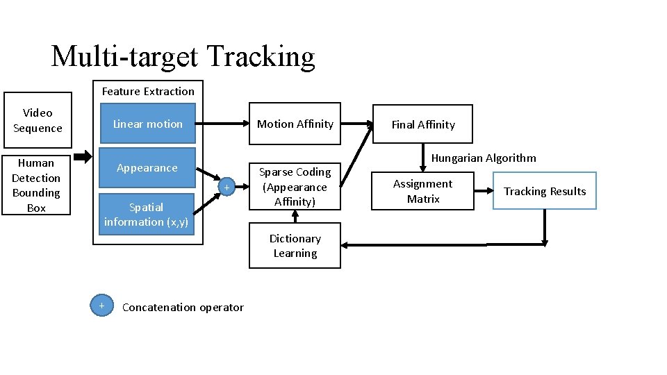
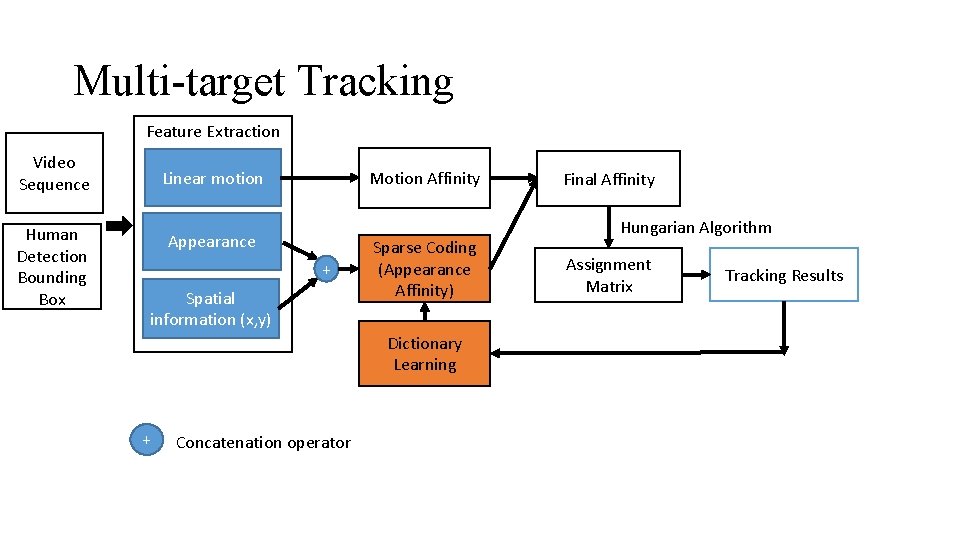
Multi-target Tracking Feature Extraction Video Sequence Human Detection Bounding Box Linear motion Motion Affinity Appearance + Spatial information (x, y) Sparse Coding (Appearance Affinity) Dictionary Learning + Concatenation operator Final Affinity Hungarian Algorithm Assignment Matrix Tracking Results

Multi-target Tracking Feature Extraction Video Sequence Human Detection Bounding Box Linear motion Motion Affinity Appearance + Spatial information (x, y) Sparse Coding (Appearance Affinity) Dictionary Learning + Concatenation operator Final Affinity Hungarian Algorithm Assignment Matrix Tracking Results

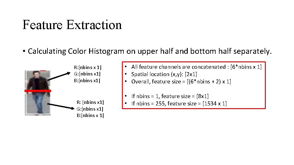
Feature Extraction • Calculating Color Histogram on upper half and bottom half separately. R: [nbins x 1] G: [nbins x 1] B: [nbins x 1] • All feature channels are concatenated : [6*nbins x 1] • Spatial location (x, y): [2 x 1] • Overall, feature size = [(6*nbins + 2) x 1] • If nbins = 1, feature size = [8 x 1] • If nbins = 255, feature size = [1534 x 1]

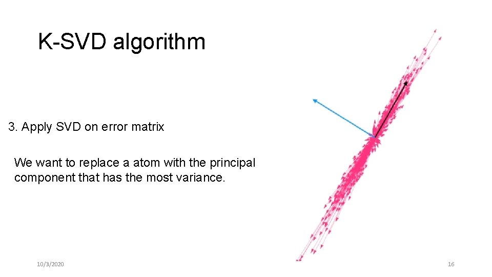
K-SVD algorithm 3. Apply SVD on error matrix We want to replace a atom with the principal component that has the most variance. 10/3/2020 16

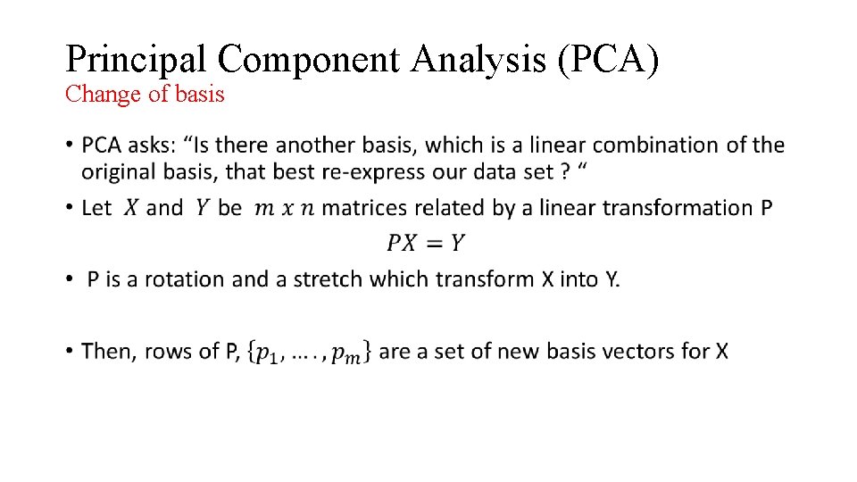
Principal Component Analysis (PCA) Change of basis •

Principal Component Analysis (PCA) Change of basis •

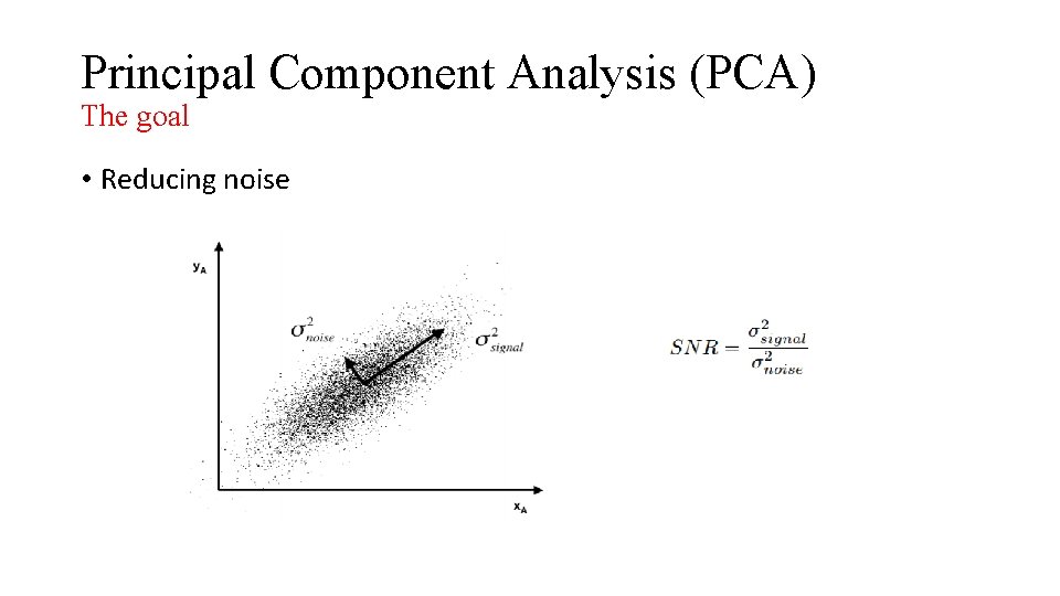
Principal Component Analysis (PCA) The goal • Reducing noise

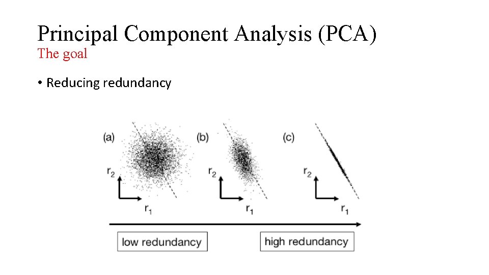
Principal Component Analysis (PCA) The goal • Reducing redundancy

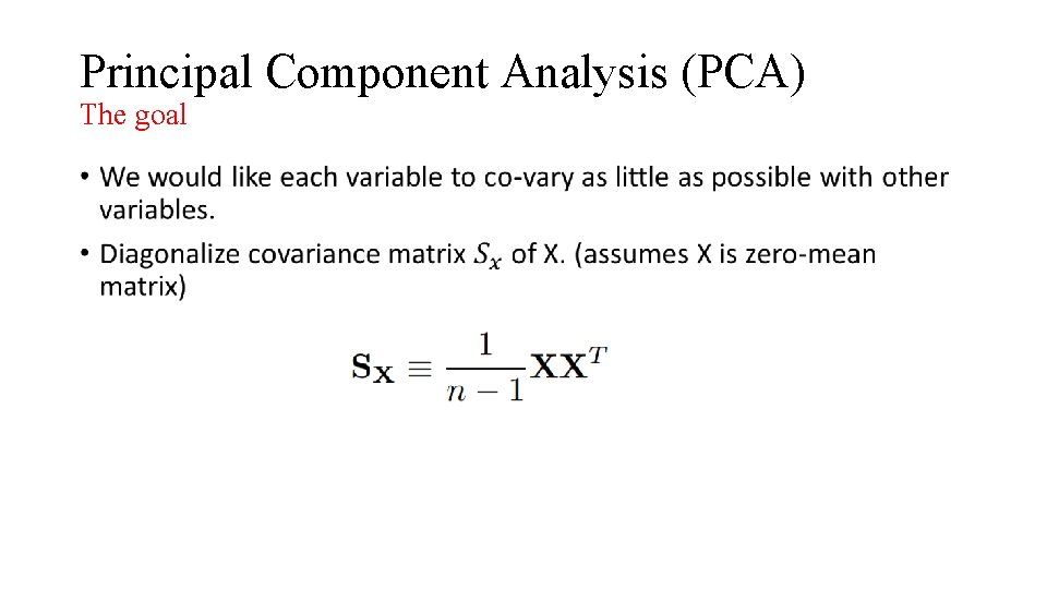
Principal Component Analysis (PCA) The goal •

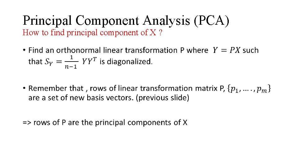
Principal Component Analysis (PCA) How to find principal component of X ? •

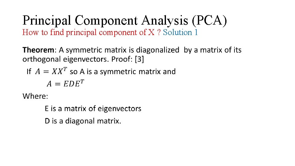
Principal Component Analysis (PCA) How to find principal component of X ? Solution 1 •

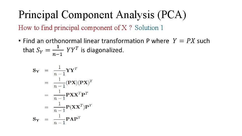
Principal Component Analysis (PCA) How to find principal component of X ? Solution 1 •

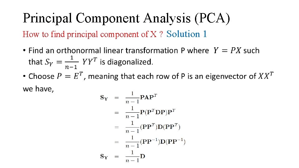
Principal Component Analysis (PCA) How to find principal component of X ? Solution 1 •

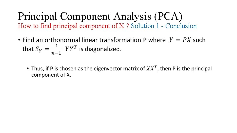
Principal Component Analysis (PCA) How to find principal component of X ? Solution 1 - Conclusion •

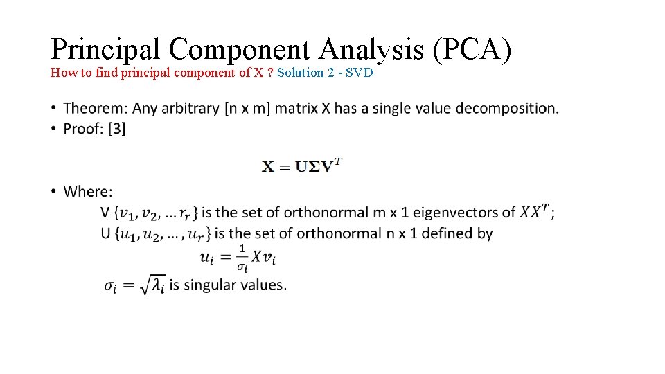
Principal Component Analysis (PCA) How to find principal component of X ? Solution 2 - SVD •

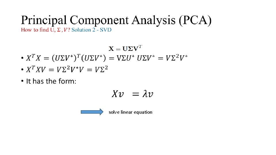
• solve linear equation

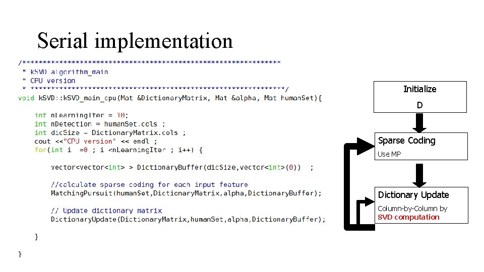
Serial implementation Initialize D Sparse Coding Use MP Dictionary Update Column-by-Column by SVD computation

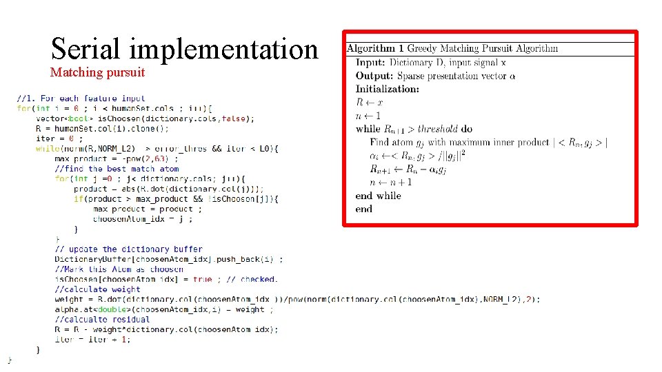
Serial implementation Matching pursuit

Serial implementation Learning Dictionary

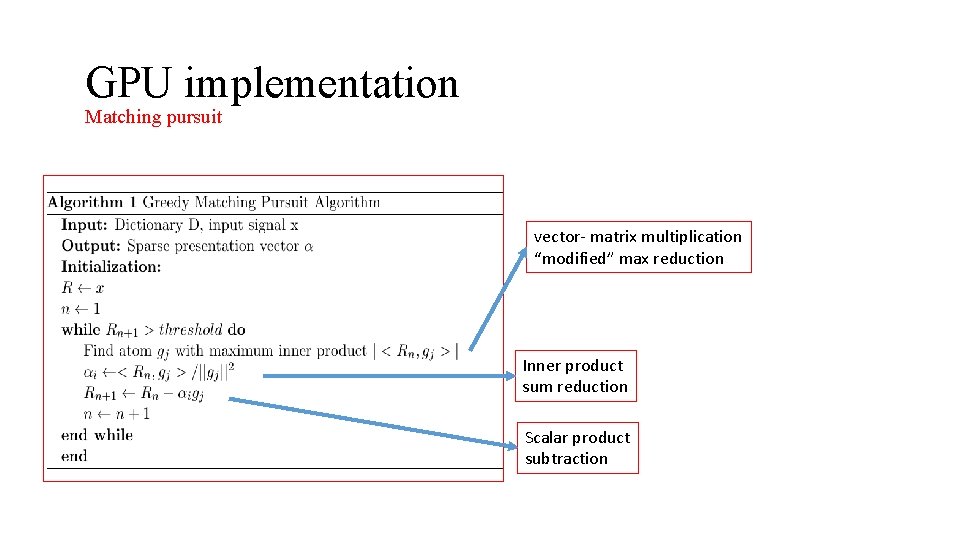
GPU implementation Matching pursuit vector- matrix multiplication “modified” max reduction Inner product sum reduction Scalar product subtraction

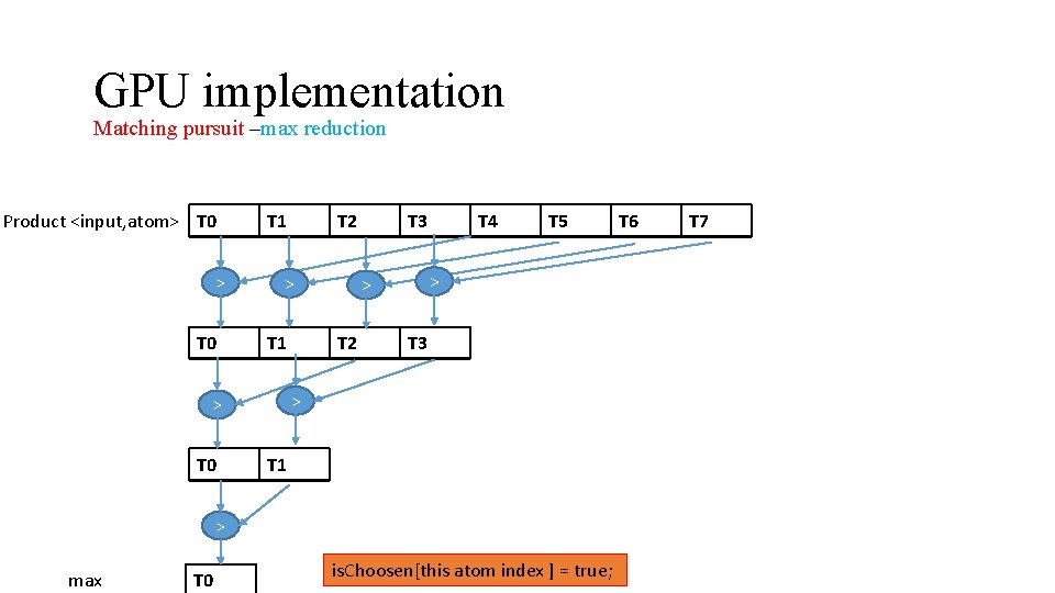
GPU implementation Matching pursuit –max reduction Product <input, atom> T 0 T 1 > T 1 T 3 T 5 > > T 2 T 4 T 3 > > T 0 T 2 T 1 > max T 0 is. Choosen[this atom index ] = true; T 6 T 7

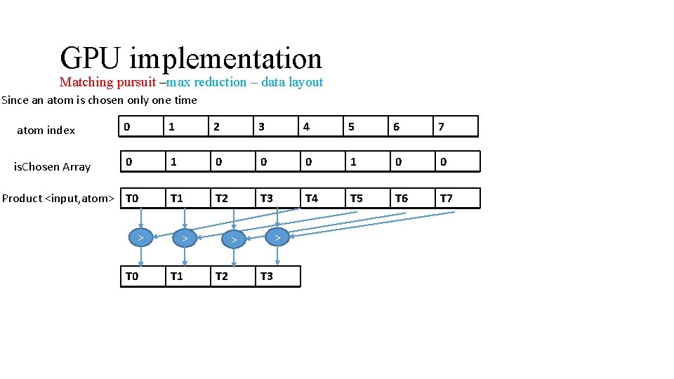
GPU implementation Matching pursuit –max reduction – data layout Since an atom is chosen only one time atom index 0 1 2 3 4 5 6 7 is. Chosen Array 0 1 0 0 T 1 T 2 T 3 T 4 T 5 T 6 T 7 Product <input, atom> T 0 > T 1 > > T 2 T 3

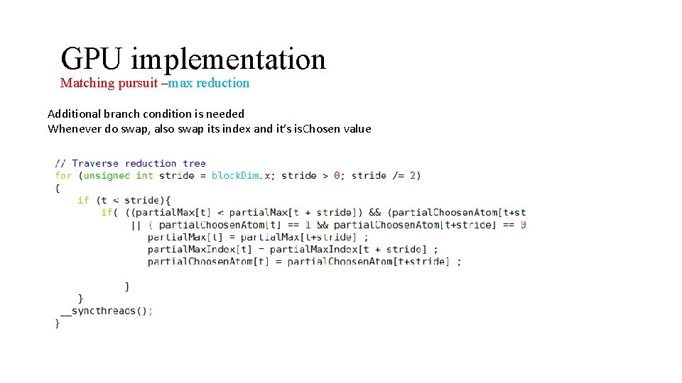
GPU implementation Matching pursuit –max reduction Additional branch condition is needed Whenever do swap, also swap its index and it’s is. Chosen value

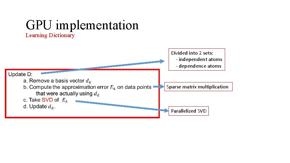
GPU implementation Learning Dictionary Divided into 2 sets: - independent atoms - dependence atoms Sparse matrix multiplication Parallelized SVD

GPU implementation Learning Dictionary Divided into 2 sets: - independent atoms - dependence atoms Sparse matrix multiplication Parallelized SVD

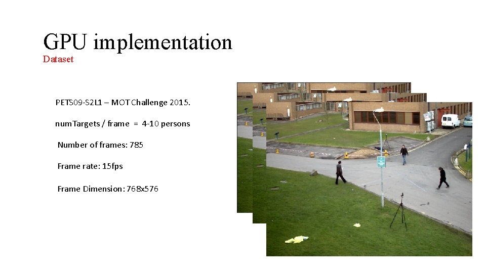
GPU implementation Dataset PETS 09 -S 2 L 1 – MOT Challenge 2015. num. Targets / frame = 4 -10 persons Number of frames: 785 Frame rate: 15 fps Frame Dimension: 768 x 576

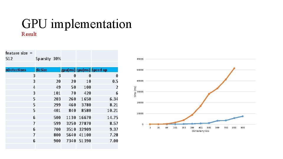
GPU implementation Result feature size = 512 Sparsity 30% dic. Size 3 3 4 3 5 5 5 6 7 6 gpu(ms) cpu(ms) Speed up 3 20 49 101 203 299 401 500 599 700 800 900 0 20 50 70 260 460 840 1130 3250 3510 5640 7340 0 10 100 420 1650 3780 8580 16670 27870 32909 41100 51390 50000 0 0. 5 2 6 6. 34 8. 21 10. 21 14. 75 8. 57 9. 37 7. 28 7. 00 40000 time (ms) n. Detections 60000 30000 20000 10000 0 3 20 49 101 203 299 401 500 Dictionary Size 599 700 800 900

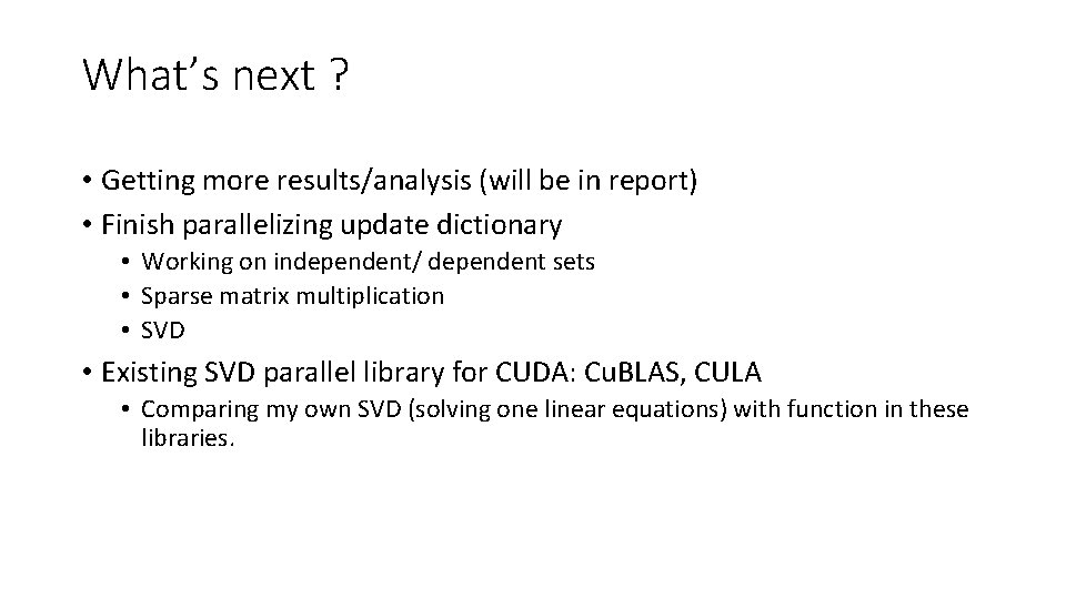
What’s next ? • Getting more results/analysis (will be in report) • Finish parallelizing update dictionary • Working on independent/ dependent sets • Sparse matrix multiplication • SVD • Existing SVD parallel library for CUDA: Cu. BLAS, CULA • Comparing my own SVD (solving one linear equations) with function in these libraries.

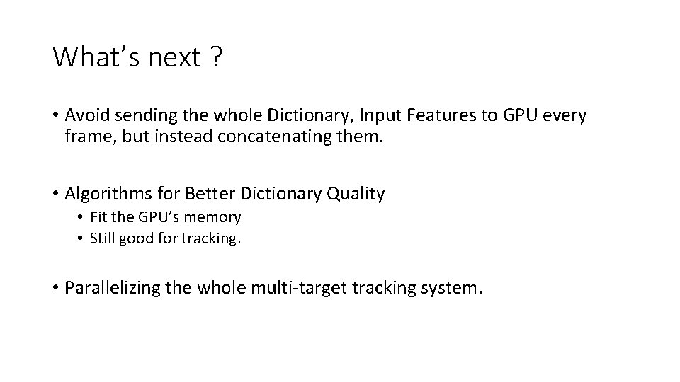
What’s next ? • Avoid sending the whole Dictionary, Input Features to GPU every frame, but instead concatenating them. • Algorithms for Better Dictionary Quality • Fit the GPU’s memory • Still good for tracking. • Parallelizing the whole multi-target tracking system.

References [1] http: //mathworld. wolfram. com/Eigen. Decomposition. Theorem. html [2] http: //stattrek. com/matrix-algebra/covariance-matrix. aspx [3] eigenvectors and SVD https: //www. cs. ubc. ca/~murphyk/Teaching/Stat 406 Spring 08/Lectures/linalg 1. pdf [4] https: //www. cs. princeton. edu/picasso/mats/PCA-Tutorial-Intuition_jp. pdf