Parallel Programming Platforms Microprocessor architecture and how to

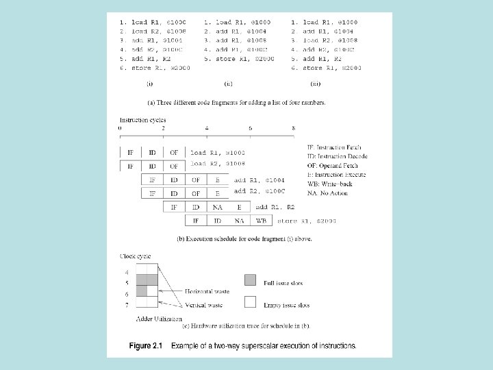
Parallel Programming Platforms • Microprocessor architecture and how to make it parallel • Pipelining, superscalar architecture • Vliw • Microprocessor memory and how to make it parallel • Caches, etc

platforms • • • Architecture Networks (ad nauseum) Cache coherence Routing Mapping processes to processors (scary)

Problems • Data dependency – Load r 1, @1000 and add r 1, @1004 – Resolved in hardware at runtime (complex) – Depends on coding style (arghh!) • Resource dependency – 2 instructions need floating point unit • Branch dependency – Speculative scheduling and rollbacks – Dynamic instruction issue (chose instructions from window)

VLIW processors • Waste lives on • Vertical -no instructions in cycle • Horizontal -parts of instructions • So use the compiler • Detect dependencies • Schedule instructions » Unroll loops, branch predictions, speculative execution

Memory problems • Memory performance • Latency • Bandwith • Cache • Faster memory between processor and dram • Cache works if there is repeated reference to same data item-temporal locality

Spatial locality

More memory tricks • Multithreading • Decreases latency • Can increase bandwith because of small cache residency • Prefetching • Advance loads • Compilers aggressively advance loads • Decreases latency, can increase bandwith • Both require more hardware

Parallel platforms • Logical organization-how programmer sees things • Control-how to express parallel tasks • Communication model-how tasks interact • Physical organization-hardware

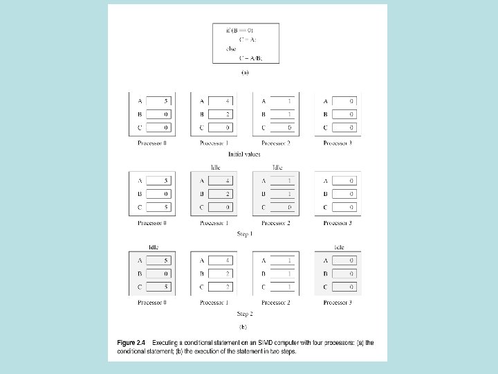
Control Structure

SIMD, MIMD, SPMD • SIMD • • Simple architecture Structured computations-arrays Early machines-Illiac IV, MPP, CM 2 Become obsolete quickly (processors change) • MIMD • Easy to build from off the shelf stuff • SPMD single program, multiple data stream

Communication Model Shared Address Space • Multiprocessors- SPMD+shared address space • UMA multicomputer-same time to access all words • NUMA multicomputer-some words take more time

Shared memory pictures

Shared memory • Read-only instructions same as serial computers • Read-write require mutual exclusion – Threads (posix) and open MP use locks • Cache coherence necessary – Serious hardware

Physical organization • PRAM, parallel random access • infinite memory, uniform access time to same memory space • Common clock, processors execute different instructions in same cycle

PRAM memory access models • EREW exclusive read exclusive write – No concurrent reads or writes – Weakest model • CREW concurrent read, exclusive write – Writes are serialized • ERCW exclusive read, concurrent write – Reads are serialized • CRCW concurrent read, concurrent write – Most powerful model, anything goes

Processor networks static and dynamic

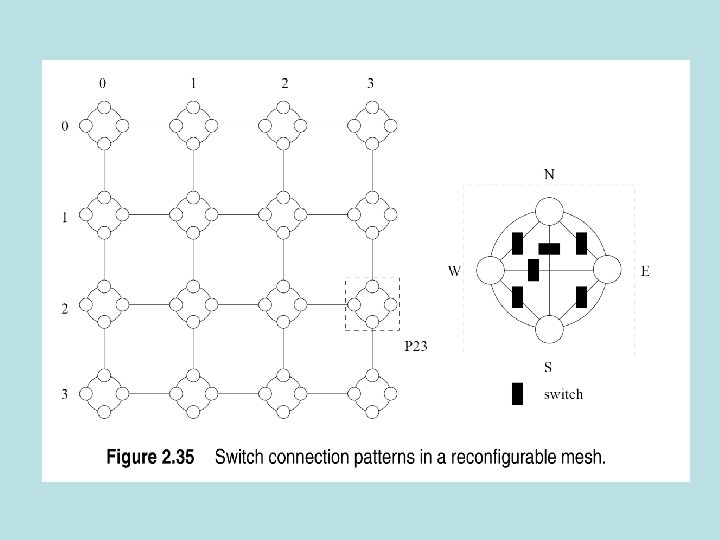
Switches and interfaces • Map input ports to output ports – Crossbars, multi-ported memory, buffer messages • Route messages • Network interfaces – – – Packetize data Routes messages Error check Buffer messages Lives on memory bus in big machines

Bus networks • Cheap • Ideal for broadcast • Shared medium limits size to dozens of nodes • Sun enterprise servers, intel pentium • Caching-reduces demand for bandwith

To cache or not to cache

Crossbar switch scales for performance, cost doesn’t scale

Multistage Network cost vs performance solution

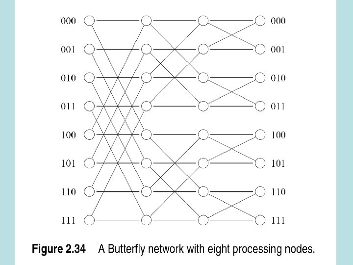
Omega network • Log p stages , p=# processing • number of inputs=number of outputs=p The perfect shuffle 2 i 0≤i≤p/2 -1 J= 2 i+1 -p p/2≤i≤p-1

The perfect shuffle picture

Omega Network • Perfect shuffle feeds p/2 switches at each stage • Each stage has 2 connection modes – Pass through – Cross over • P/2 x log p switching nodes

Omega Network

Omega Network-blocking • Path from processor 2 to memory bank 7 is blocked for other processors

Completely Connected and Star Networks • Highly realistic

Real networks

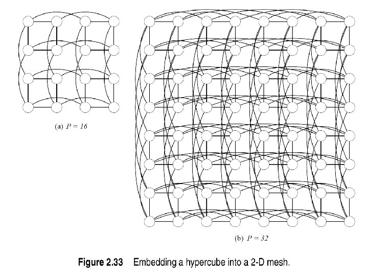
How to build a hypercube connect 2 (d-1) dimensional hypercubes to get a d dimensional hypercube

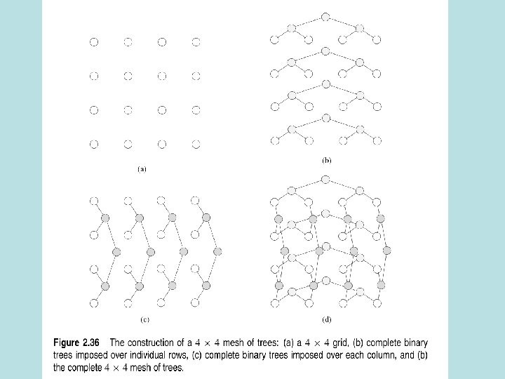
Tree Networks • Static-processors at nodes • Dynamic-switches at nodes, processors at leaves – Messages go up and down tree

Fat tree • More switches, less traffic congestion

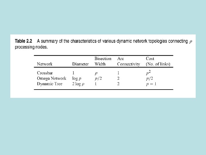
Evaluation of static networks • Diameter-max distance between 2 processing nodes » Distance is shortest path • Connectivity-how many paths between nodes? » Arc connectivity is the cut-set • Bisection width-# links to remove to get two equal size networks • Channel width-#wires on a link • Channel rate-peak bit rate for a wire • Channel bandwith-peak rate for a link • Cost-number of links or the number of wires

Static networks

Dynamic Networks • Treat switches as nodes, same definitions for diameter and connectivity • Bisection width-nodes only

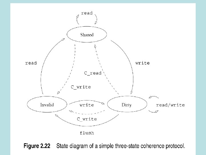
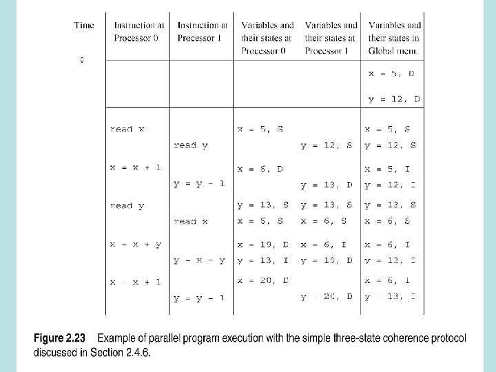
Cache coherence in multiprocessor systems • How to keep caches and memory consistent • Update-change variable in cache, update memory and remote caches (not cheap) • Invalidate-change variable, invalidate other copies (other processors might not use the variable)

Invalidate , Update

Tradeoffs and false sharing • Communication overhead of updates vs. idle time of invalidates • False sharing-different processors update different parts of same cache line • Invalidate-entire line is taken out by processor • Other processors have to import their parts from remote processor

How the invalidate protocol works • Initially x is in global memory (shared) • P 0 does a store and marks other copies invalid and marks its own as dirty. • If P 1 attempts to write to variable, P 0 first updates the variable (it becomes shared again).

Snoopy Caches – Bus-based – Each processor keeps tags for data items – Listens for reads, writes to its dirty items and takes over

Snoopy • The good-can do local mods without generating traffic • The bad-doesn’t scale to lots of processors • Summary- Bus based

Directory based • Bit map indicates state of data

Directory • Centralized directory can be a bottleneck • Distributed directory scales better • Get concurrent update possibility but • Need update messages to other processors

Communication Costs • Start-up time (ts) • Per-hop time (th) Latency-time for first bit to arrive at next node • Per-word transfer time (tw) tw=1/r, r=bandwith

Routing Store and forward, Packet routing

Cut through design goals • All packets take same path • Error information at message, not packet level • Low cost error detection methods

Cut through design • • • Flits- flow control digits Very small, 4 bits to 32 bytes Send tracer flit to establish route All flits follow thereafter Passed through intermediate nodes, not stored

Deadlock among the flits

Simple Cost Model for sending messages • Model tcomm=ts+lth+twm • Should » Communicate in bulk » Minimize amount sent » Minimize distance of transfer • Can try to do the first two

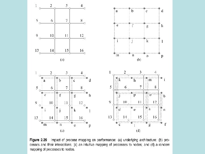
Cost model • Hard to minimize distance of transfer » Programmer has little control over process mapping » Random (two step) routing. First send to randomly selected node, then route to destination-minimizes congestion. » Th dominated by ts and tw • New model-ignore latency • Don’t think about topology when designing algorithms • Unless there is congestion

Why it is hard to model communication costs in shared address machines Programmer doesn’t control memory-the system does Cache thrashing Invalidate and update overheads hard to model Spacial locality hard to model Prefetching (done by compiler) False sharing Contention

Solution • Back of envelope model – Assume that remote access results in word being fetched into local cache – Subsume all coherence, network, memory overheads are included in ts (the access cost) – Per word access cost of tw includes cost of remote (vs local) access • Cost of sharing m words=ts+twm – The same model

Routing Algorithms • Deterministic algorithms • Adaptive algorithms • Dimension ordered routing – Next hop determined by dimension – Mesh- xy routing – Hypercube- E-cube routing

E Cube Routing • Compute Ps XOR Pd – Number of ones = minimum distance • Send message on dimension k=position of least significant bit in Ps XOR Pd • Intermediate node Pi computes Pi XOR Pd and does the same

E Cube Routing

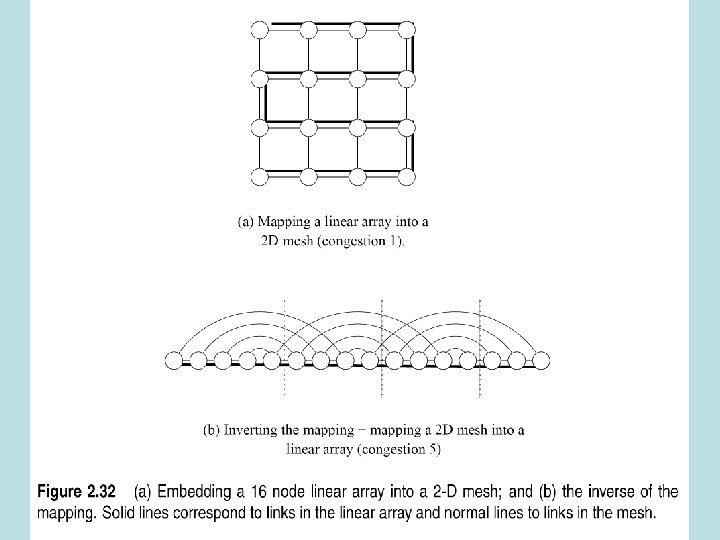
Mapping Techniques for Graphs • Why? Because you might have to port a program from one machine to another • Need to know how the communication patterns of the algorithm will be affected – Some mappings might produce congestion

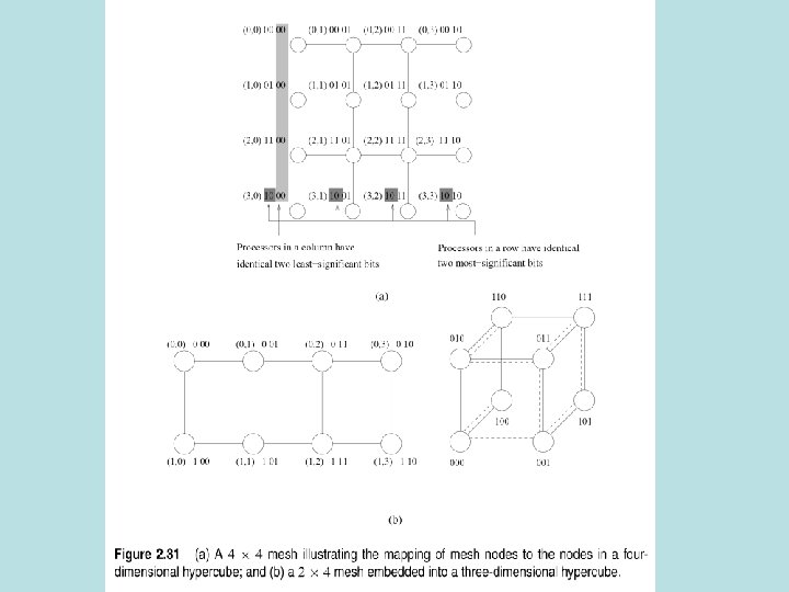
Embed Linear Array into Hypercube • Linear array of 2 d nodes • D dimensional hypercube • Map node i of linear array onto node G(i, d) of hypercube • G is the binary reflected Gray code

Mapping linear array into hypercube • Get gray code of dimension d+1 from gray code of dimension d by reflecting and prefixing (0=old, 1=new)