Parallel Programming Chapter 3 Introduction to Parallel Architectures


 = (n) • Claim:")
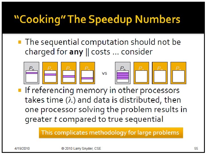
 • Unfortunately, the best speedup possible for most")
 > n • Most texts besides")
 • Selim Akl has given a multitude of examples that establish that")
 – Real life situations such as a driveway which a person can")
 • The last chapter of Akl’s textbook and several journal papers by")
 = ts/tp • A bound on")
/p time processors Shows nontrivial parallel algorithm’s computation component")
 time processors Shows a nontrivial parallel algorithm’s communication component")
/p + (n, p) time processors Combining these, we")

 is Cost = Parallel")


 • For algorithms for traditional problems, superlinearity is")


 has lower complexity than (n)/p (i.")


 • Takes the opposite approach of Amdahl’s Law – Amdahl’s law")


- Slides: 97
Parallel Programming Chapter 3 Introduction to Parallel Architectures Johnnie Baker January 26 , 2011 1
References • The PDF slides (i. e. , ones with the black stripe across the top) were created by Larry Snyder, co-author of text: http: //www. cs. washington. edu/education/courses/524/08 wi/ • Calvin Lin and Lawrence Snyder, Principles of Parallel Programming, Addison Wesley, 2009 (Textbook) • Johnnie Baker, Slides for course, Parallel & Distributed Processing, http: //www. cs. kent. edu/~jbaker/PDC-F 08/ • Selim Akl, Parallel Computations: Models & Methods, Prentice Hall, 1997. • Michael Quinn, Parallel Programming in C with MPI and Open. MP, Mc. Graw Hill, 2004.
Skip this Slide
Skip this Slide
Skip this Slide
Skip this Slide
Skip this Slide
SKIP - Not Assigned
SKIP - Not Assigned
Additional Slides on Performance Analysis Johnnie Baker Course taught in Fall 2010 Parallel & Distributed Processing Chapter 7: Performance Analysis http: //www. cs. kent. edu/~jbaker/PDC-F 10/
References • • Slides are from my Fall 2010 “Parallel and Distributed Computing” course at website http: //www. cs. kent. edu/~jbaker/PDC-F 10/ (Primary Reference): Selim Akl, “Parallel Computation: Models and Methods”, Prentice Hall, 1997, Updated online version available through website. (Secondary Reference) Michael Quinn, Parallel Programming in C with MPI and Open MP, Ch. 7, Mc. Graw Hill, 2004. (Course Textbook PDC-F 10 Barry Wilkinson and Michael Allen, “Parallel Programming: Techniques and Applications Using Networked Workstations and Parallel Computers ”, Prentice Hall, First Edition 1999 or Second Edition 2005, Chapter 1. 65
Outline • • Speedup Superlinearity Issues Speedup Analysis Cost Efficiency Amdahl’s Law Gustafson’s Law and Gustafson-Baris’s Law Amdahl Effect 66
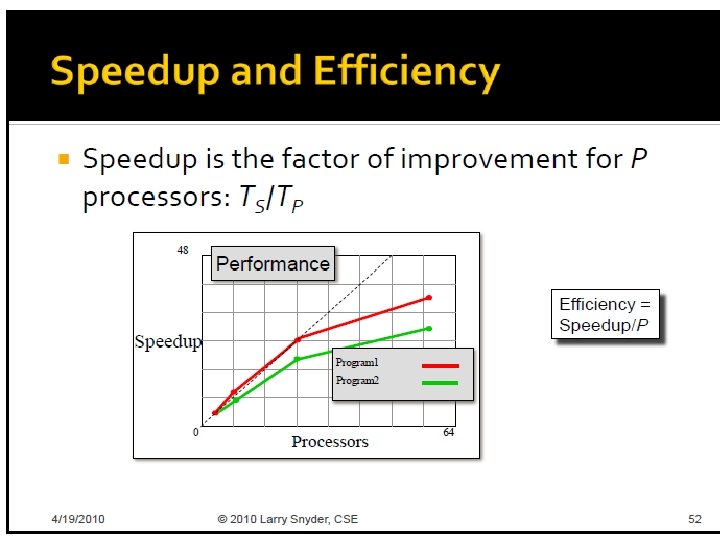
Speedup • • Speedup measures increase in running time due to parallelism. The number of PEs is given by n. S(n) = ts/tp , where – – ts is the running time on a single processor, using the fastest known sequential algorithm tp is the running time using a parallel processor. 67
Linear Speedup Usually Optimal • Speedup is linear if S(n) = (n) • Claim: The maximum possible speedup for parallel computers with n PEs is n. • Usual Argument: (Assume ideal conditions) – Assume a computation is partitioned perfectly into n processes of equal duration. – Assume no overhead is incurred as a result of this partitioning of the computation – (e. g. , partitioning process, information passing, coordination of processes, etc), – Under these ideal conditions, the parallel computation will execute n times faster than the sequential computation and • the parallel running time will be ts /n. – Then the parallel speedup in this “ideal situation” is S(n) = ts /(ts /n) = n 68
Linear Speedup Normally Less than Optimal) • Unfortunately, the best speedup possible for most applications is much smaller than n – The “ideal conditions” performance mentioned in earlier argument is usually unattainable. – Normally, some parts of programs are sequential and allow only one PE to be active. – Sometimes a significant number of processors are idle for certain portions of the program. • During parts of the execution, many PEs may be waiting to receive or to send data. • E. g. , congestion may occur in message passing 69
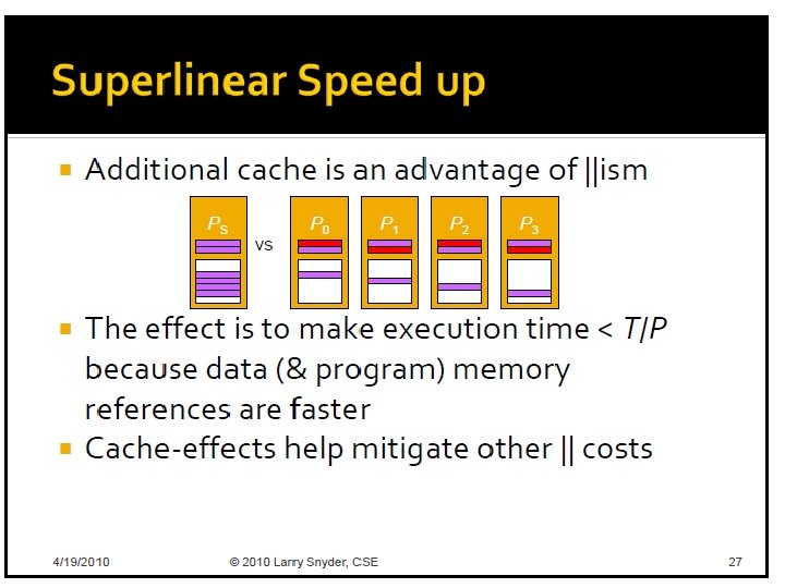
Superlinear Speedup • Superlinear speedup occurs when S(n) > n • Most texts besides Akl’s argue that – Linear speedup is the maximum speedup obtainable. • The earlier argument is used as a “proof” that superlinearity is always impossible. – Occasionally speedup that appears to be superlinear may occur, but can be explained by other reasons such as • the extra memory in parallel system. • a sub-optimal sequential algorithm is compared to parallel algorithm. • “Luck”, in case of algorithm that has a random aspect in its design (e. g. , random selection) 70
Superlinearity (cont) • Selim Akl has given a multitude of examples that establish that superlinear algorithms are required for many non-standard problems, such as – Problems where meeting deadlines is a part of the problem requirements – Problems where not all of the data is initially available, but has to be processed as it arrives and prior to the arrival of the next set of data. • E. g. , sensor data which arrives at regular intervals. – Problems where too many conditions must be satisfied simultaneously in order to gain security access using either a sequential computer or even a parallel computer without a required minimum number of processors 71
Superlinearity (cont) – Real life situations such as a driveway which a person can only keep a driveway open during a severe snowstorm with the help of several friends. • If a problem either cannot be solved in the required amount of time or cannot be solved at all by a sequential computer, it seems fair to say that ts=. • However, then , S(n) = ts/tp = > 1, so it seems reasonable to consider these solutions to be “superlinear”.
Superlinearity (cont) • The last chapter of Akl’s textbook and several journal papers by Professor Selim Akl were written to establish that superlinearity can occur. – It may still be a long time before the possibility of superlinearity occurring is fully accepted. – Superlinearity has long been a hotly debated topic and is unlikely to be widely accepted quickly – even when theoretical evidence is provided. • For more details on superlinearity, see “Parallel Computation: Models and Methods”, Selim Akl, pgs 14 -20 (Speedup Folklore Theorem) and Chapter 12. 73
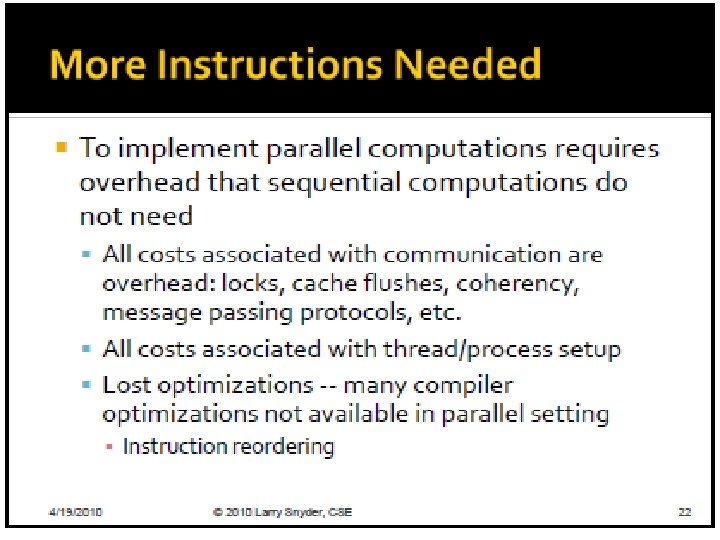
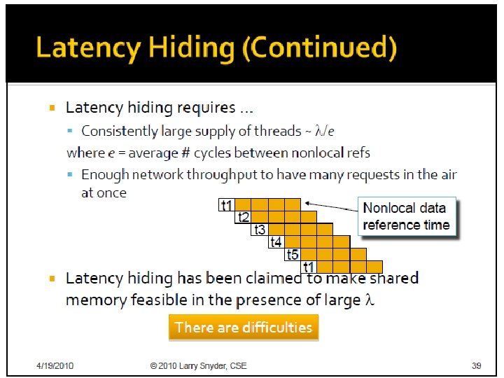
Speedup Analysis • Recall speedup definition: S(n, p) = ts/tp • A bound on the maximum speedup is given by – – Inherently sequential computations are (n) Potentially parallel computations are (n) Communication operations are (n, p) The “≤” bound above is due to the fact that the communications cost is not the only overhead in the parallel computation. 74
Execution time for parallel portion (n)/p time processors Shows nontrivial parallel algorithm’s computation component as a decreasing function of the number of processors used. 75
Time for communication (n, p) time processors Shows a nontrivial parallel algorithm’s communication component as an increasing function of the number of processors. 76
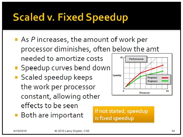
Execution Time of Parallel Portion (n)/p + (n, p) time processors Combining these, we see for a fixed problem size, there is an optimum number of processors that minimizes overall execution time. 77
Speedup Plot “elbowing out” speedup processors 78
Cost • The cost of a parallel algorithm (or program) is Cost = Parallel running time #processors • Since “cost” is a much overused word, the term “algorithm cost” is sometimes used for clarity. • The cost of a parallel algorithm should be compared to the running time of a sequential algorithm. – Cost removes the advantage of parallelism by charging for each additional processor. – A parallel algorithm whose cost is big-oh of the running time of an optimal sequential algorithm is called cost-optimal. 79
Cost Optimal • From last slide, a parallel algorithm is optimal if parallel cost = O(f(t)), where f(t) is the running time of an optimal sequential algorithm. • Equivalently, a parallel algorithm for a problem is said to be cost-optimal if its cost is proportional to the running time of an optimal sequential algorithm for the same problem. – By proportional, we means that cost tp n = k ts where k is a constant and n is nr of processors. • In cases where no optimal sequential algorithm is known, then the “fastest known” sequential algorithm is sometimes used instead. 80
Efficiency 81
Bounds on Efficiency • Recall (1) • For algorithms for traditional problems, superlinearity is not possible and (2) speedup ≤ processors • Since speedup ≥ 0 and processors > 1, it follows from the above two equations that 0 (n, p) 1 • Algorithms for non-traditional problems also satisfy 0 (n, p). However, for superlinear algorithms, it follows that (n, p) > 1 since speedup > p. 82
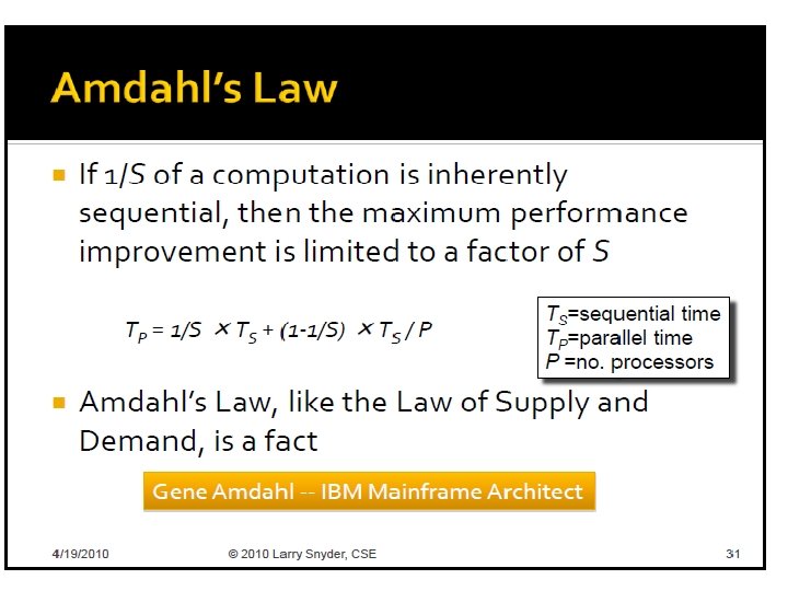
Amdahl’s Law Let f be the fraction of operations in a computation that must be performed sequentially, where 0 ≤ f ≤ 1. The maximum speedup achievable by a parallel computer with n processors is • The word “law” is often used by computer scientists when it is an observed phenomena (e. g, Moore’s Law) and not a theorem that has been proven in a strict sense. • However, a formal argument is given on the next slide that shows Amdahl’s law is valid for “traditional problems”. • The diagram used in this proof is from the textbook by Wilkinson and Allen (See References). 83
Usual Argument: If the fraction of the computation that cannot be divided into concurrent tasks is f, and no overhead incurs when the computation is divided into concurrent parts, the time to perform the computation with n processors is given by tp ≥ fts + [(1 - f )ts] / n, as shown below: 84
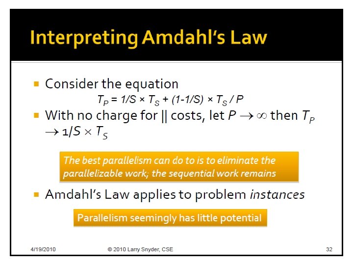
Amdahl’s Law • Preceding argument assumes that speedup can not be superliner; i. e. , S(n) = ts/ tp n – Assumption only valid for traditional problems. – Question: Where is this assumption used? • The pictorial portion of this argument is taken from chapter 1 of Wilkinson and Allen • Sometimes Amdahl’s law is just stated as S(n) 1/f • Note that S(n) never exceeds 1/f and approaches 1/f as n increases. 85
Consequences of Amdahl’s Limitations to Parallelism • For a long time, Amdahl’s law was viewed as a fatal flaw to the usefulness of parallelism. – Some computer professionals not in a high performance computing area still believe this. • Amdahl’s law is valid for traditional problems and has several useful interpretations. • Some textbooks show Amdahl’s law can be used to increase the efficient of parallel algorithms – See Reference (16), Jordan & Alaghband textbook • Amdahl’s law shows that efforts required to further reduce the fraction of the code that is sequential may pay off in huge performance gains. • Hardware that achieves even a small decrease in the percent of things executed sequentially may be considerably more 86 efficient.
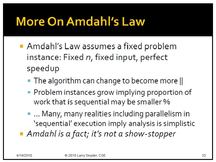
Limitations of Amdahl’s Law – A key flaw in past arguments that Amdahl’s law is a fatal limit to the future of parallelism is • Gustafon’s Law: The proportion of the computations that are sequential normally decreases as the problem size increases. – Note: “Gustafon’s law” is a simplified version of the Gustafon. Barsis Law – Other limitations in applying Amdahl’s Law: • Its proof focuses on the steps in a particular algorithm, and does not consider whether other algorithms with more parallelism may exist • Amdahl’s law applies only to ‘standard’ problems were superlinearity cannot occur 87
Amdahl’s Law - Example 1 • 95% of a program’s execution time occurs inside a loop that can be executed in parallel. What is the maximum speedup we should expect from a parallel version of the program executing on 8 CPUs? 88
Amdahl’s Law - Example 2 • 5% of a parallel program’s execution time is spent within inherently sequential code. • The maximum speedup achievable by this program, regardless of how many PEs are used, is 89
Amdahl’s Law - Self Quiz • An oceanographer gives you a serial program and asks you how much faster it might run on 8 processors. You can only find one function amenable to a parallel solution. Benchmarking on a single processor reveals 80% of the execution time is spent inside this function. What is the best speedup a parallel version is likely to achieve on 8 processors? Show that the answer is about 3. 3 90
Amdahl Effect • Typically communications time (n, p) has lower complexity than (n)/p (i. e. , time for parallel part) • As n increases, (n)/p dominates (n, p) • As n increases, – sequential portion of algorithm decreases – speedup increases • Amdahl Effect: Speedup is usually an increasing function of the problem size. 91
Illustration of Amdahl Effect Speedup n = 10, 000 n = 100 Processors 92
Amdahl’s Law Summary • Treats problem size as a constant • Shows how execution time decreases as number of processors increases • Amdahl Effect: Normally, as the problem size increases, the sequential portion of the problem decreases and the speedup increases • It is generally accepted by HPC professionals that Amdahl’s law is not a serious limit to the benefits and future of parallel computing. 93
Gustafson-Barsis’s Law Formal Statement: Given a parallel program of size n using p processors, let f denote the fraction of the total execution time spent in the serial code. The maximum speedup S achievable by this program is S p - (p-1)s • A much more optimistic law than Amdahl’s, but still does not allow superlinearity. • Using the parallel computation as a starting point rather than sequential computation, it allows the problem size to be an increasing function of the number of processors • Because it uses the parallel computation as the starting point, the speedup predicted is referred to as scaled speedup
Gustafson-Barsis Law (Cont) • Takes the opposite approach of Amdahl’s Law – Amdahl’s law determines speedup by using a serial computation to predict how quickly the computation could be done on multiple processors. – Gustafson-Barsis’s law begins with a parallel computation and estimates how much faster the parallel computation is than the same computation executing on a parallel processor.
Gustafon-Barsis Law Example: An application on 64 processors requires 220 seconds to run. Benchmarking revels that 5 percent of the time is spent executing sequential portions of the computation on a single processor. What is the scaled speedup of the application. • Since f = 0. 05, the scaled speedup on 64 processors is S = 64 – (64 -1)0. 05 = 64 – 3. 15 = 60. 85
Homework for Ch. 3 1. 2. 3. 4. 5. 6. 7. 8. 9. (7. 2 -Quinn) Starting with the definition of efficiency, prove that if p’>p, then (n, p’) (n, p). (7. 4 - Quinn): Benchmarking of a sequential program revels that 95% of the execution time is spent inside functions that are amendable to parallelization. What is the maximum speedup that we could expect from executing a parallel version of this program on 10 processors? (7. 5 - Quinn) For a problem size of interest, 6% of the operations of a parallel program are inside I/O functions that are executed on a single processor. What is the minimum number of processors needed in order for the parallel program to exhibit a speedup of 10? (7. 7 Quinn) Shauna’s program achieves a speedup of 9 on 10 processors. What is the maximum fraction of computation that may consist of inherently sequential operations. ? (7. 8 -Quinn) Brandon’s parallel program executes in 242 seconds on 16 processors. Through benchmarking, he determines that 9 seconds is spend performing initializations and cleanup on one processor. During the remaining 233 seconds, all 16 processors are active. What is the scaled speedup achieved by Brandon’s program. Cortney benchmarks one of her parallel programs executing on 40 processors. She discovers it spends 99% of its time inside parallel code. What is the scaled speedup of her program. (7. 11 – Quinn) Both Amdahl’s law and Gustafson-Barsis’s law are derived from the same general speedup formula. However, when increasing the number of processors p , the maximum speedup predicted by Amdahl’s law converges on 1/f, while the speedup predicted by Gustafson-Barsis’s law increases without bound. Explain why this is so. (3. 2 –Lin/Snyder) Should contention be considered a special part of overhead? Can there be contention in a single-threaded program? Explain. (3. 5 - Lin/Snyder) Describe a parallel computation whose speedup does not increase with