Parallel Processing Neural Networks on SIMDGPU Architectures CSC

Parallel Processing Neural Networks on SIMD/GPU Architectures CSC 7551 Derek Kern December 8 th, 2011

Quick Apology a. I have 80 slides and ~75 minutes b. So, we are going to move pretty fast c. I apologize in advance d. However, I have lots of information to convey e. Hopefully, it will be worth it

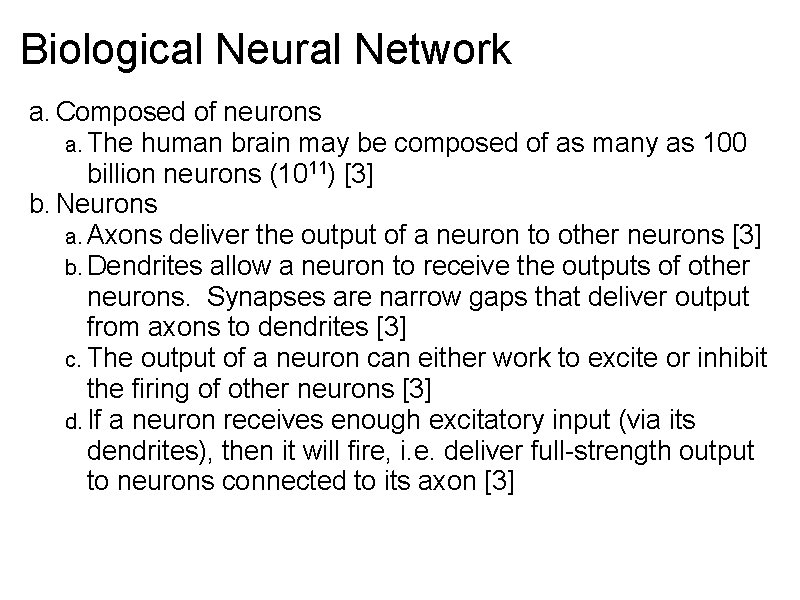
Biological Neural Network a. Composed of neurons a. The human brain may be composed of as many as 100 billion neurons (1011) [3] b. Neurons a. Axons deliver the output of a neuron to other neurons [3] b. Dendrites allow a neuron to receive the outputs of other neurons. Synapses are narrow gaps that deliver output from axons to dendrites [3] c. The output of a neuron can either work to excite or inhibit the firing of other neurons [3] d. If a neuron receives enough excitatory input (via its dendrites), then it will fire, i. e. deliver full-strength output to neurons connected to its axon [3]

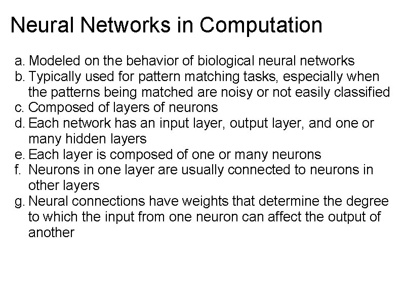
Neural Networks in Computation a. Modeled on the behavior of biological neural networks b. Typically used for pattern matching tasks, especially when the patterns being matched are noisy or not easily classified c. Composed of layers of neurons d. Each network has an input layer, output layer, and one or many hidden layers e. Each layer is composed of one or many neurons f. Neurons in one layer are usually connected to neurons in other layers g. Neural connections have weights that determine the degree to which the input from one neuron can affect the output of another

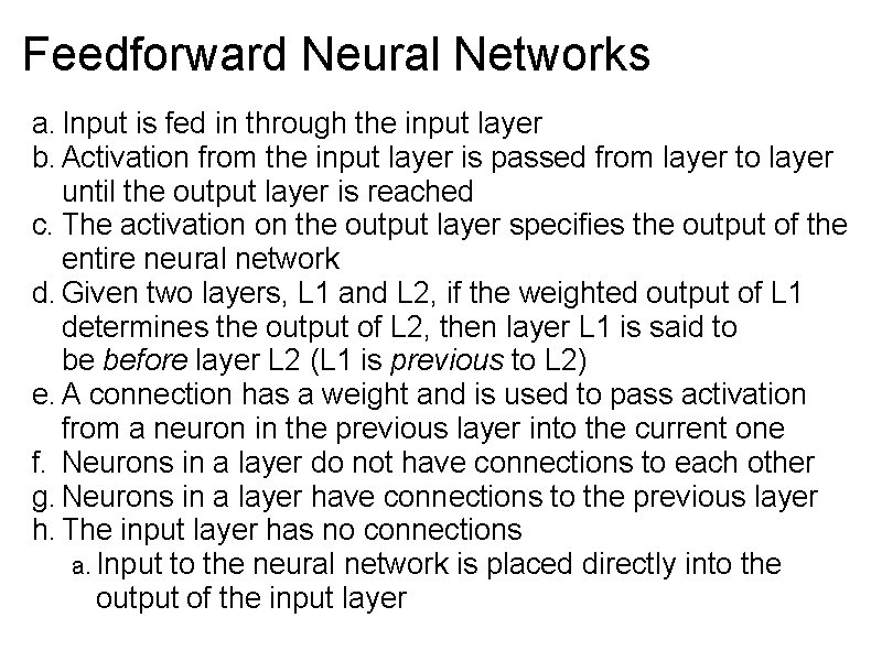
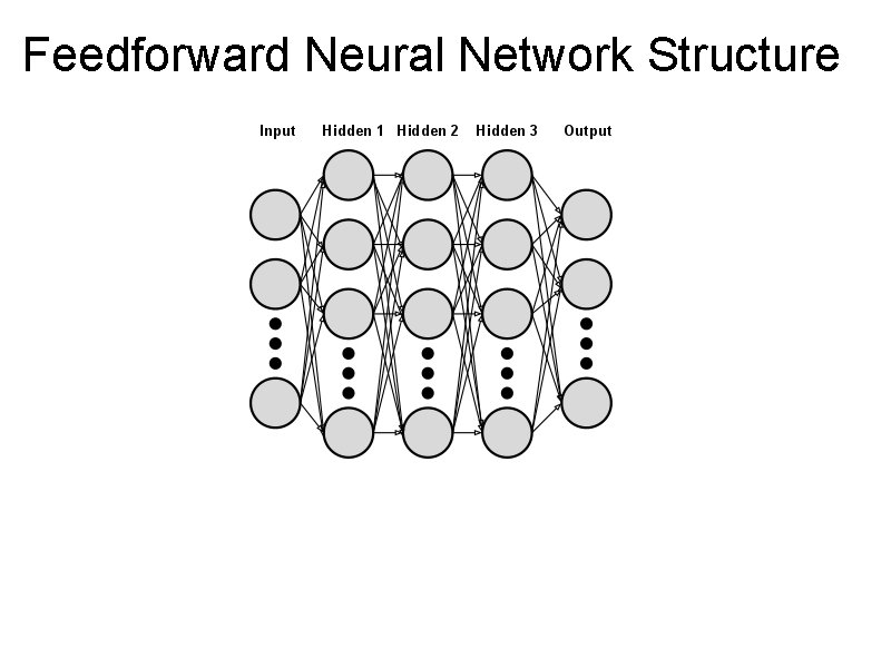
Feedforward Neural Networks a. Input is fed in through the input layer b. Activation from the input layer is passed from layer to layer until the output layer is reached c. The activation on the output layer specifies the output of the entire neural network d. Given two layers, L 1 and L 2, if the weighted output of L 1 determines the output of L 2, then layer L 1 is said to be before layer L 2 (L 1 is previous to L 2) e. A connection has a weight and is used to pass activation from a neuron in the previous layer into the current one f. Neurons in a layer do not have connections to each other g. Neurons in a layer have connections to the previous layer h. The input layer has no connections a. Input to the neural network is placed directly into the output of the input layer

Feedforward Neural Network Structure

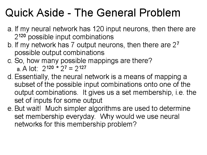
Quick Aside - The General Problem a. If my neural network has 120 input neurons, then there are 2120 possible input combinations b. If my network has 7 output neurons, then there are 27 possible output combinations c. So, how many possible mappings are there? a. A lot: 2120 * 27 = 2127 d. Essentially, the neural network is a means of mapping a subset of the possible input combinations onto one of the output combinations. It gives us a set membership, i. e. the set of inputs for some output e. But wait! Much simpler algorithms are used to determine set membership everyday. Why would we use neural networks for this membership problem?

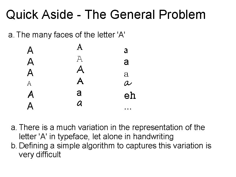
Quick Aside - The General Problem a. The many faces of the letter 'A' A A A A A a a a eh. . . a. There is a much variation in the representation of the letter 'A' in typeface, let alone in handwriting b. Defining a simple algorithm to captures this variation is very difficult

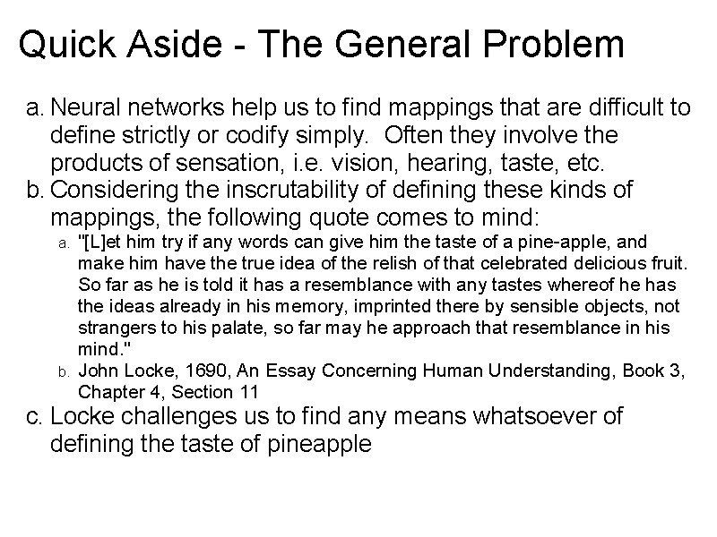
Quick Aside - The General Problem a. Neural networks help us to find mappings that are difficult to define strictly or codify simply. Often they involve the products of sensation, i. e. vision, hearing, taste, etc. b. Considering the inscrutability of defining these kinds of mappings, the following quote comes to mind: "[L]et him try if any words can give him the taste of a pine-apple, and make him have the true idea of the relish of that celebrated delicious fruit. So far as he is told it has a resemblance with any tastes whereof he has the ideas already in his memory, imprinted there by sensible objects, not strangers to his palate, so far may he approach that resemblance in his mind. " b. John Locke, 1690, An Essay Concerning Human Understanding, Book 3, Chapter 4, Section 11 a. c. Locke challenges us to find any means whatsoever of defining the taste of pineapple

Quick Aside - The General Problem a. Jerry Fodor (1981) offers a challenge similar to Locke's a. How does one define the (transitive verb) 'to paint'? b. How about 'X covers Y with paint'? a. But, what if a paint factory explodes covering passers-by with paint? c. How about 'X paints Y if and only if X is an agent and X covers Y with paint'? a. But, what if I kicked a bucket of paint, thereby covering my shoes with paint? d. How about 'X paints Y if and only if X is an agent and X intentionally covers Y with paint'? a. Does Michelangelo paint his brush when he covers it with paint?

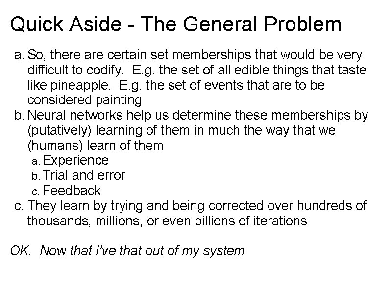
Quick Aside - The General Problem a. So, there are certain set memberships that would be very difficult to codify. E. g. the set of all edible things that taste like pineapple. E. g. the set of events that are to be considered painting b. Neural networks help us determine these memberships by (putatively) learning of them in much the way that we (humans) learn of them a. Experience b. Trial and error c. Feedback c. They learn by trying and being corrected over hundreds of thousands, millions, or even billions of iterations OK. Now that I've that out of my system

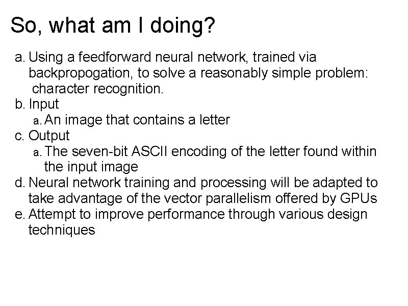
So, what am I doing? a. Using a feedforward neural network, trained via backpropogation, to solve a reasonably simple problem: character recognition. b. Input a. An image that contains a letter c. Output a. The seven-bit ASCII encoding of the letter found within the input image d. Neural network training and processing will be adapted to take advantage of the vector parallelism offered by GPUs e. Attempt to improve performance through various design techniques

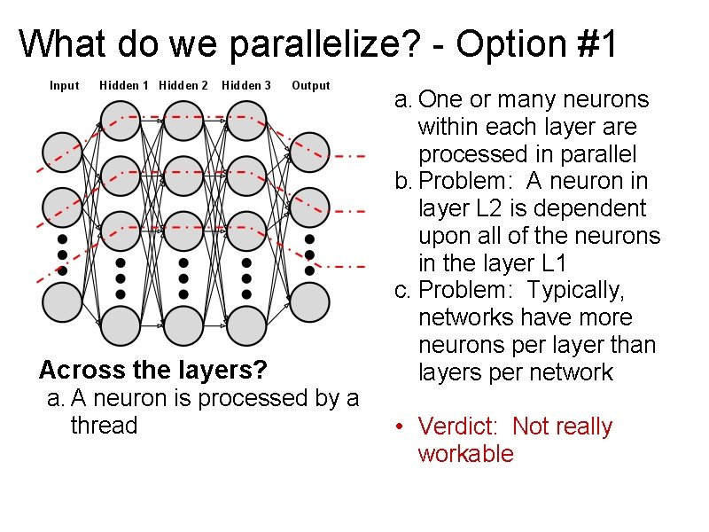
What do we parallelize? - Option #1 Across the layers? a. A neuron is processed by a thread a. One or many neurons within each layer are processed in parallel b. Problem: A neuron in layer L 2 is dependent upon all of the neurons in the layer L 1 c. Problem: Typically, networks have more neurons per layer than layers per network • Verdict: Not really workable

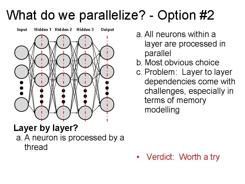
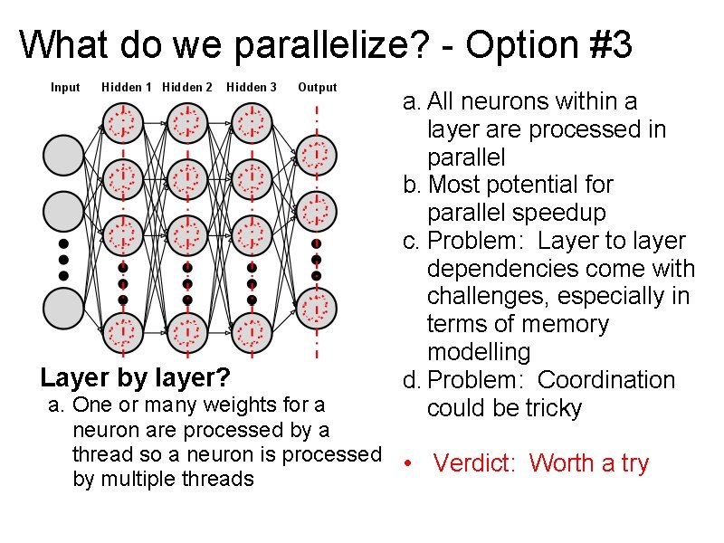
What do we parallelize? - Option #2 a. All neurons within a layer are processed in parallel b. Most obvious choice c. Problem: Layer to layer dependencies come with challenges, especially in terms of memory modelling Layer by layer? a. A neuron is processed by a thread • Verdict: Worth a try

What do we parallelize? - Option #3 Layer by layer? a. All neurons within a layer are processed in parallel b. Most potential for parallel speedup c. Problem: Layer to layer dependencies come with challenges, especially in terms of memory modelling d. Problem: Coordination could be tricky a. One or many weights for a neuron are processed by a thread so a neuron is processed • Verdict: Worth a try by multiple threads

I know this sounds strange, but. . . a. I want to describe why vector parallelization of neural networks may not be a good idea b. Consider parallelization Option #2, where neurons within each layer are processed in parallel c. Each of these neurons are dependent upon each and every neuron in the previous layer so they each will need to read the output of each neuron in that layer d. If layer L 2 is being processed, then all of the threads processing the neurons of L 2 must be able to concurrently read the outputs of all of the neurons of L 1 e. So, we are virtually assured to have memory access collisions that limit the parallel processing speedup

But, on the other hand. . . a. The computations necessary to determine the output of each neuron just look like they should be done in parallel b. Depending upon the size of the network, each neuron may need tens of thousands of small, relatively simple, roughly identical operations. And this only refers to the input-output processing, not network training which is of the same structure and more computationally intensive c. Thus, if the dependency problem is overwhelmed by the parallel benefit or can be mitigated, then it will have been shown that this is precisely the type of computation for which vector architectures are well-suited • So, we'll give it a try

Two faces of the neural network a. Processing (Feedforward) a. Outputting results based upon inputs b. Feedforward process is responsible for turning input values on the input layer into output values on the output layer c. Activation is passed from the input layer, through the hidden layers, and on to the output layer b. Training (Backpropogation) a. Teaching the network to respond to a pattern of input with a pattern of output b. Backpropogation process is responsible for training the network c. Feedforward is used for initial network population during backpropogation

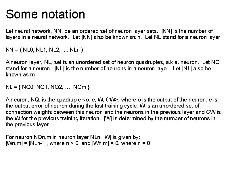
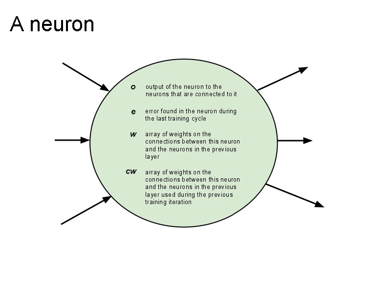
Some notation Let neural network, NN, be an ordered set of neuron layer sets. |NN| is the number of layers in a neural network. Let |NN| also be known as n. Let NL stand for a neuron layer NN = ( NL 0, NL 1, NL 2, . . . , NLn ) A neuron layer, NL, set is an unordered set of neuron quadruples, a. k. a. neuron. Let NQ stand for a neuron. |NL| is the number of neurons in a neuron layer. Let |NL| also be known as m NL = { NQ 0, NQ 1, NQ 2, …, NQm } A neuron, NQ, is the quadruple <o, e, W, CW>, where o is the output of the neuron, e is the output error of neuron during the last training cycle, W is an unordered set of connection weights between this neuron and the neurons in the previous layer and CW is the W for the previous training iteration. |W| is determined by the number of neurons in the previous layer For neuron NQn, m in neuron layer NLn, |W| is given by: |Wn, m| = |NLn-1|, where n > 0; and |Wn, m| = 0, where n = 0

A neuron

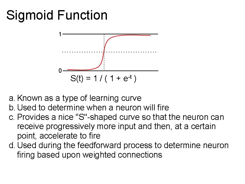
Sigmoid Function S(t) = 1 / ( 1 + e-t ) a. Known as a type of learning curve b. Used to determine when a neuron will fire c. Provides a nice "S"-shaped curve so that the neuron can receive progressively more input and then, at a certain point, accelerate to fire d. Used during the feedforward process to determine neuron firing based upon weighted connections

Algorithm Feedforward Algorithm Feed. Forward( neuron_outputs, neuron_weights, inputs ): neuron_outputs[n][m]; neuron_weights[n][m][w]; inputs[m]; sum = 0. 0; /* Put the inputs onto the input layer */ For j : = 0 step 1 until |NL 0| - 1 neuron_outputs[0][j] : = inputs[j]; /* Set outputs for all neurons based upon inputs */ For i : = 1 step 1 until |NN| - 1 For j : = 0 step 1 until |NLi| - 1 For k : = 0 step 1 until |NLi-1| - 1 sum : = sum + ( neuron_outputs[i - 1][k] * neuron_weights[i][j][k] ); neuron_outputs[i][j] : = 1 / ( 1 + exp( -sum ) ); /* sigmoid on the sum */

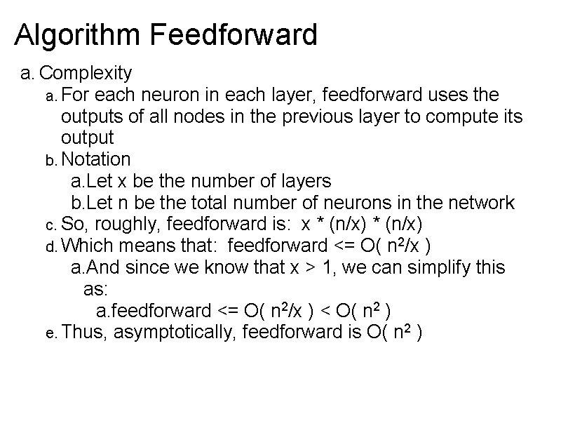
Algorithm Feedforward a. Complexity a. For each neuron in each layer, feedforward uses the outputs of all nodes in the previous layer to compute its output b. Notation a. Let x be the number of layers b. Let n be the total number of neurons in the network c. So, roughly, feedforward is: x * (n/x) d. Which means that: feedforward <= O( n 2/x ) a. And since we know that x > 1, we can simplify this as: a. feedforward <= O( n 2/x ) < O( n 2 ) e. Thus, asymptotically, feedforward is O( n 2 )

Algorithm Backpropogation( neuron_outputs, neuron_errors, neuron_weights, c_neuron_weight, inputs, desired_outputs, learning_momentum, learning_rate ): neuron_outputs[n][m]; neuron_errors[n][m]; neuron_weights[n][m][w]; c_neuron_weights[n][m][w]; /* weights cached from previous training */ desired_outputs[m]; inputs[m]; learning_rate; learning_momentum; sum : = 0. 0; Feed. Forward( neuron_outputs, neuron_weights, inputs ); /* Set the deltas for the output layer according to the desired outputs */ For j : = 0 step 1 until |NL|NN|-1| - 1 neuron_errors[|NN|-1][j] : = neuron_outputs[|NN|-1][j] * ( 1 - neuron_outputs[|NN|-1][j] ) * ( desired_outputs[j] - neuron_outputs[|NN|-1][j] );

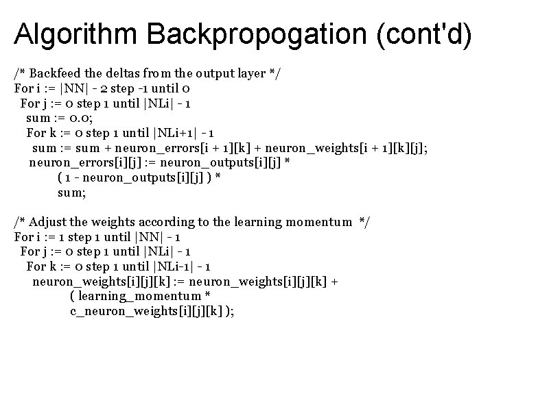
Algorithm Backpropogation (cont'd) /* Backfeed the deltas from the output layer */ For i : = |NN| - 2 step -1 until 0 For j : = 0 step 1 until |NLi| - 1 sum : = 0. 0; For k : = 0 step 1 until |NLi+1| - 1 sum : = sum + neuron_errors[i + 1][k] + neuron_weights[i + 1][k][j]; neuron_errors[i][j] : = neuron_outputs[i][j] * ( 1 - neuron_outputs[i][j] ) * sum; /* Adjust the weights according to the learning momentum */ For i : = 1 step 1 until |NN| - 1 For j : = 0 step 1 until |NLi| - 1 For k : = 0 step 1 until |NLi-1| - 1 neuron_weights[i][j][k] : = neuron_weights[i][j][k] + ( learning_momentum * c_neuron_weights[i][j][k] );

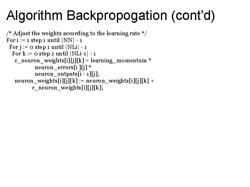
Algorithm Backpropogation (cont'd) /* Adjust the weights according to the learning rate */ For i : = 1 step 1 until |NN| - 1 For j : = 0 step 1 until |NLi| - 1 For k : = 0 step 1 until |NLi-1| - 1 c_neuron_weights[i][j][k] = learning_momentum * neuron_errors[i ][j] * neuron_outputs[i - 1][j]; neuron_weights[i][j][k] : = neuron_weights[i][j][k] + c_neuron_weights[i][j][k];

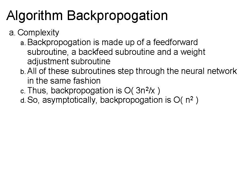
Algorithm Backpropogation a. Complexity a. Backpropogation is made up of a feedforward subroutine, a backfeed subroutine and a weight adjustment subroutine b. All of these subroutines step through the neural network in the same fashion c. Thus, backpropogation is O( 3 n 2/x ) d. So, asymptotically, backpropogation is O( n 2 )

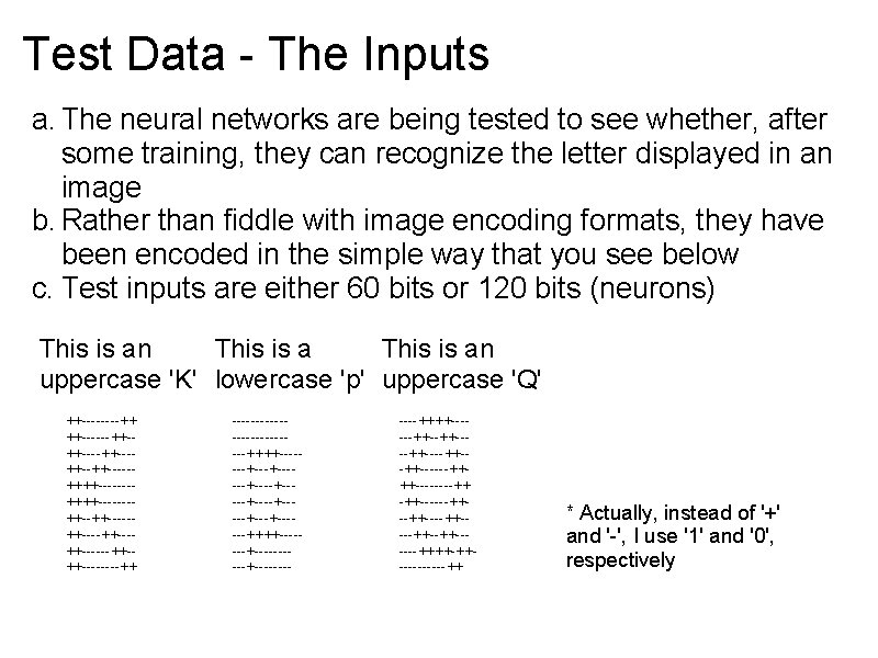
Test Data - The Inputs a. The neural networks are being tested to see whether, after some training, they can recognize the letter displayed in an image b. Rather than fiddle with image encoding formats, they have been encoded in the simple way that you see below c. Test inputs are either 60 bits or 120 bits (neurons) This is an uppercase 'K' lowercase 'p' uppercase 'Q' ++----++ ++------++-++---++-----++++-------++-----++---++------++-++----++ -------------++++-------+------+----+-----+------++++----------+----++++------++----++--++------++++----++ -++------++----++--++------++++-++-----++ * Actually, instead of '+' and '-', I use '1' and '0', respectively

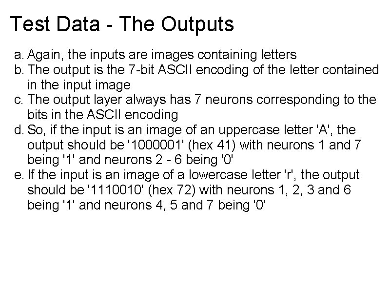
Test Data - The Outputs a. Again, the inputs are images containing letters b. The output is the 7 -bit ASCII encoding of the letter contained in the input image c. The output layer always has 7 neurons corresponding to the bits in the ASCII encoding d. So, if the input is an image of an uppercase letter 'A', the output should be '1000001' (hex 41) with neurons 1 and 7 being '1' and neurons 2 - 6 being '0' e. If the input is an image of a lowercase letter 'r', the output should be '1110010' (hex 72) with neurons 1, 2, 3 and 6 being '1' and neurons 4, 5 and 7 being '0'

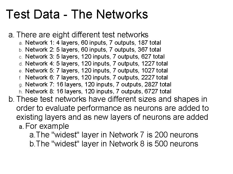
Test Data - The Networks a. There are eight different test networks a. b. c. d. e. f. g. h. Network 1: 4 layers, 60 inputs, 7 outputs, 187 total Network 2: 5 layers, 60 inputs, 7 outputs, 367 total Network 3: 5 layers, 120 inputs, 7 outputs, 627 total Network 4: 5 layers, 120 inputs, 7 outputs, 1227 total Network 5: 7 layers, 120 inputs, 7 outputs, 1027 total Network 6: 7 layers, 120 inputs, 7 outputs, 2227 total Network 7: 16 layers, 120 inputs, 7 outputs, 2827 total Network 8: 16 layers, 120 inputs, 7 outputs, 6727 total b. These test networks have different sizes and shapes in order to evaluate performance as neurons are added to existing layers and as new layers of neurons are added a. For example a. The "widest" layer in Network 7 is 200 neurons b. The "widest" layer in Network 8 is 500 neurons

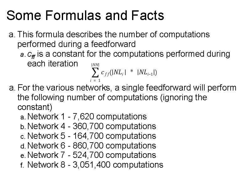
Some Formulas and Facts a. This formula describes the number of computations performed during a feedforward a. cff is a constant for the computations performed during each iteration a. For the various networks, a single feedforward will perform the following number of computations (ignoring the constant) a. Network 1 - 7, 620 computations b. Network 4 - 360, 700 computations c. Network 5 - 164, 700 computations d. Network 6 - 860, 700 computations e. Network 7 - 524, 700 computations f. Network 8 - 3, 051, 400 computations

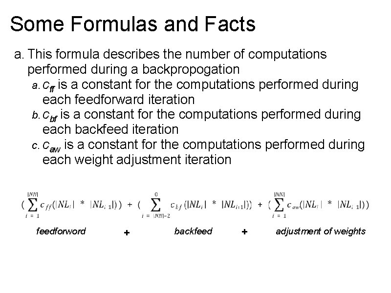
Some Formulas and Facts a. This formula describes the number of computations performed during a backpropogation a. cff is a constant for the computations performed during each feedforward iteration b. cbf is a constant for the computations performed during each backfeed iteration c. caw is a constant for the computations performed during each weight adjustment iteration feedforword + backfeed + adjustment of weights

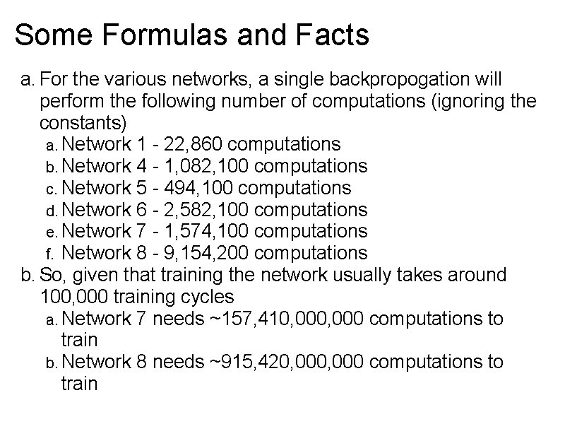
Some Formulas and Facts a. For the various networks, a single backpropogation will perform the following number of computations (ignoring the constants) a. Network 1 - 22, 860 computations b. Network 4 - 1, 082, 100 computations c. Network 5 - 494, 100 computations d. Network 6 - 2, 582, 100 computations e. Network 7 - 1, 574, 100 computations f. Network 8 - 9, 154, 200 computations b. So, given that training the network usually takes around 100, 000 training cycles a. Network 7 needs ~157, 410, 000 computations to train b. Network 8 needs ~915, 420, 000 computations to train

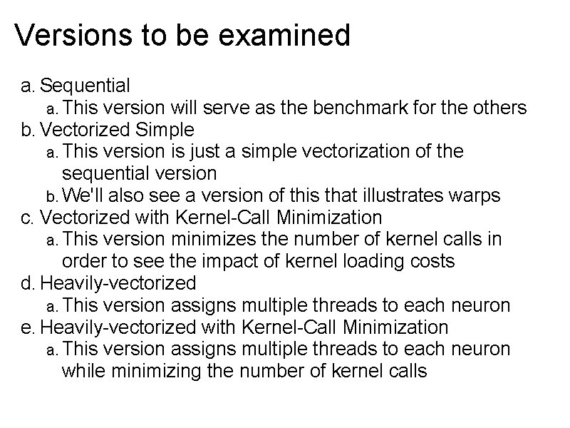
Versions to be examined a. Sequential a. This version will serve as the benchmark for the others b. Vectorized Simple a. This version is just a simple vectorization of the sequential version b. We'll also see a version of this that illustrates warps c. Vectorized with Kernel-Call Minimization a. This version minimizes the number of kernel calls in order to see the impact of kernel loading costs d. Heavily-vectorized a. This version assigns multiple threads to each neuron e. Heavily-vectorized with Kernel-Call Minimization a. This version assigns multiple threads to each neuron while minimizing the number of kernel calls

Versions to be examined (cont'd) a. . And a few minor versions (and instructive failures) • Note: When examining the implementation ideas behind each version, my explanations will largely focus on feedforward (even though the idea will be implemented everywhere possible)

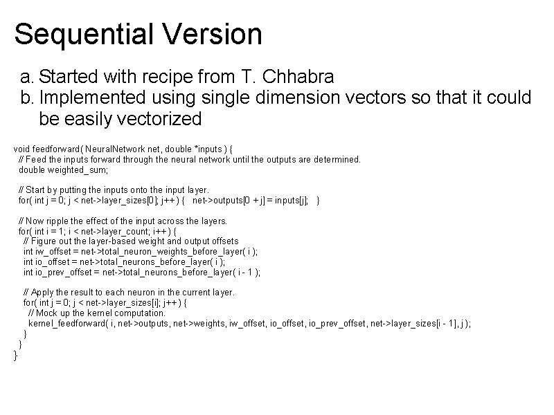
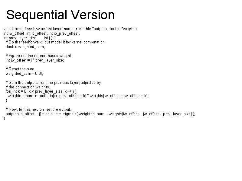
Sequential Version a. Started with recipe from T. Chhabra b. Implemented usingle dimension vectors so that it could be easily vectorized void feedforward( Neural. Network net, double *inputs ) { // Feed the inputs forward through the neural network until the outputs are determined. double weighted_sum; // Start by putting the inputs onto the input layer. for( int j = 0; j < net->layer_sizes[0]; j++ ) { net->outputs[0 + j] = inputs[j]; } // Now ripple the effect of the input across the layers. for( int i = 1; i < net->layer_count; i++ ) { // Figure out the layer-based weight and output offsets int iw_offset = net->total_neuron_weights_before_layer( i ); int io_offset = net->total_neurons_before_layer( i ); int io_prev_offset = net->total_neurons_before_layer( i - 1 ); // Apply the result to each neuron in the current layer. for( int j = 0; j < net->layer_sizes[i]; j++ ) { // Mock up the kernel computation. kernel_feedforward( i, net->outputs, net->weights, iw_offset, io_prev_offset, net->layer_sizes[i - 1], j ); } } }

Sequential Version void kernel_feedforward( int layer_number, double *outputs, double *weights, int iw_offset, int io_prev_offset, int prev_layer_size, int j ) { // Do the feedforward, but model it for kernel computation. double weighted_sum; // Figure out the neuron-based weight int jw_offset = j * prev_layer_size; // Reset the sum. weighted_sum = 0. 0 f; // Sum the outputs from the previous layer, adjusted by // the connection weights. for( int k = 0; k < prev_layer_size; k++ ) { weighted_sum += outputs[io_prev_offset + k] * weights[iw_offset + jw_offset + k]; } // Now, for this neuron, set the outputs[io_offset + j] = calculate_sigmoid( weighted_sum + weights[iw_offset + jw_offset + prev_layer_size] ); }

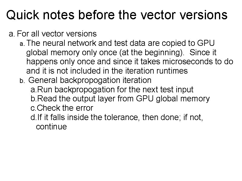
Quick notes before the vector versions a. For all vector versions a. The neural network and test data are copied to GPU global memory only once (at the beginning). Since it happens only once and since it takes microseconds to do and it is not included in the iteration runtimes b. General backpropogation iteration a. Run backpropogation for the next test input b. Read the output layer from GPU global memory c. Check the error d. If it falls inside the tolerance, then done; if not, continue

Quick notes before the vector versions a. For all vector versions (cont'd) a. General feedforward iteration a. Run forward for the next test input b. Read the output layer from GPU global memory c. Write out the result

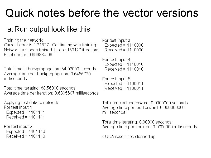
Quick notes before the vector versions a. Run output look like this Training the network: For test input 3 Current error is 1. 21327. Continuing with training. . . Expected = 1110000 Network has been trained. It took 130127 iterations. Received = 1110000 Final error is 9. 99988 e-06 For test input 4 Expected = 1110010 Total time in backpropogation: 84. 02000 seconds Received = 1110010 Average time per backpropogation: 0. 6456720 milliseconds For test input 5 Expected = 1100011 Total time iterating: 88. 56000 seconds Received = 1100011 Average time per iteration: 0. 6805607 milliseconds Applying test data to network: For test input 1 Expected = 1101111 Received = 1101111 For test input 2 Expected = 1101110 Received = 1101110 Total time in feedforward: 0. 0000000 seconds Average time per feedforward: 0. 00000 milliseconds Total time iterating: 0. 00000 seconds Average time per iteration: 0. 0000000 milliseconds CUDA resources cleaned up

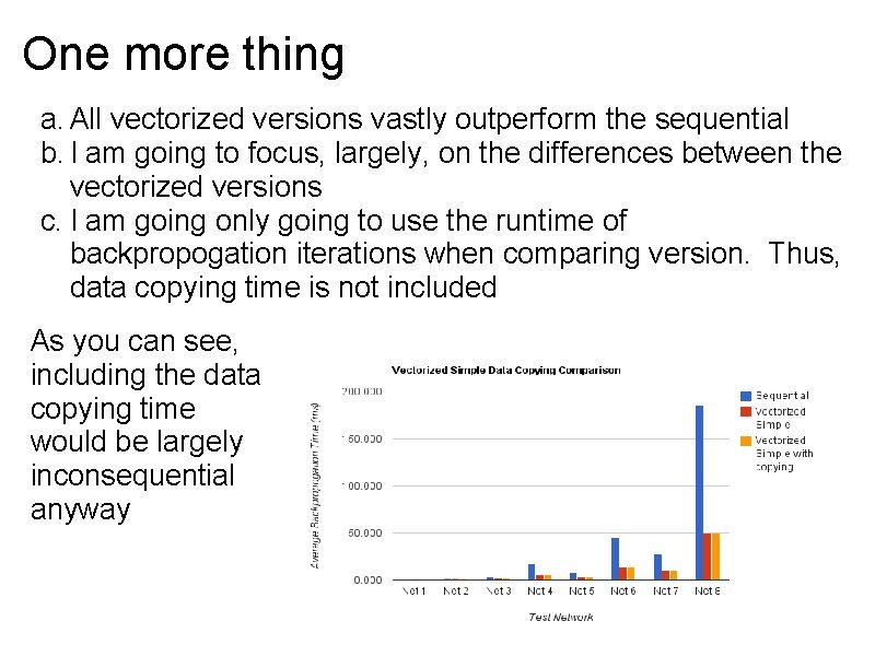
One more thing a. All vectorized versions vastly outperform the sequential b. I am going to focus, largely, on the differences between the vectorized versions c. I am going only going to use the runtime of backpropogation iterations when comparing version. Thus, data copying time is not included As you can see, including the data copying time would be largely inconsequential anyway

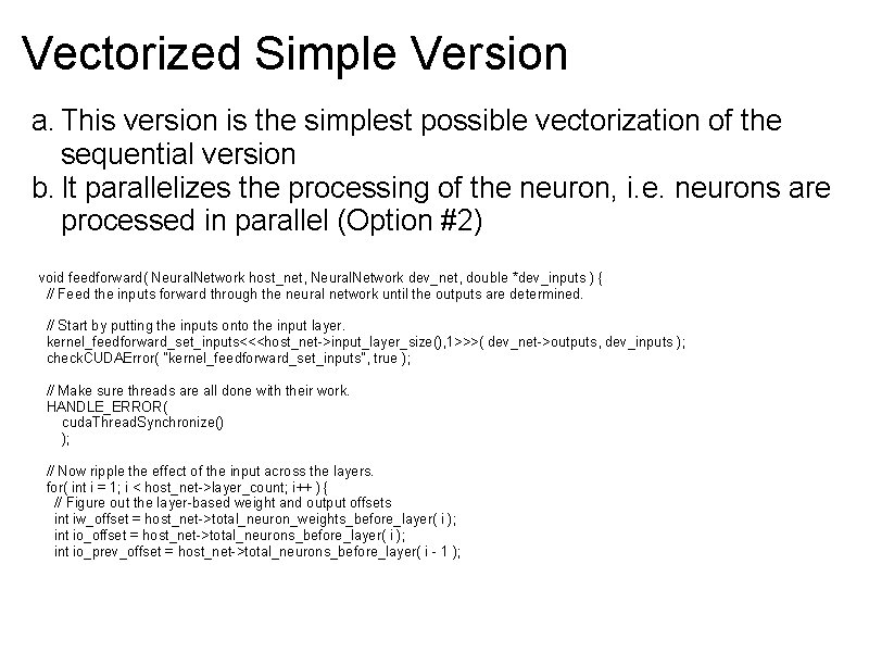
Vectorized Simple Version a. This version is the simplest possible vectorization of the sequential version b. It parallelizes the processing of the neuron, i. e. neurons are processed in parallel (Option #2) void feedforward( Neural. Network host_net, Neural. Network dev_net, double *dev_inputs ) { // Feed the inputs forward through the neural network until the outputs are determined. // Start by putting the inputs onto the input layer. kernel_feedforward_set_inputs<<<host_net->input_layer_size(), 1>>>( dev_net->outputs, dev_inputs ); check. CUDAError( "kernel_feedforward_set_inputs", true ); // Make sure threads are all done with their work. HANDLE_ERROR( cuda. Thread. Synchronize() ); // Now ripple the effect of the input across the layers. for( int i = 1; i < host_net->layer_count; i++ ) { // Figure out the layer-based weight and output offsets int iw_offset = host_net->total_neuron_weights_before_layer( i ); int io_offset = host_net->total_neurons_before_layer( i ); int io_prev_offset = host_net->total_neurons_before_layer( i - 1 );

Vectorized Simple Version // Do the kernel computation. kernel_feedforward<<<host_net->layer_sizes[i], 1>>>( dev_net->outputs, dev_net->weights, iw_offset, io_offset, io_prev_offset, host_net->layer_sizes[i - 1] ); check. CUDAError( "kernel_feedforward", true ); // Make sure threads are all done with their work. HANDLE_ERROR( cuda. Thread. Synchronize() ); } } __global__ void kernel_feedforward( double *outputs, double *weights, int iw_offset, int io_prev_offset, int prev_layer_size ) { // Do the feedforward, but model it for kernel computation. double weighted_sum = 0. 0 f; int j = block. Idx. x; // Figure out the neuron-based weight int jw_offset = j * prev_layer_size; // Sum the outputs from the previous layer, adjusted by the connection weights. for( int k = 0; k < prev_layer_size; k++ ) { weighted_sum += outputs[io_prev_offset + k] * weights[iw_offset + jw_offset + k]; } // Now, for this neuron, set the outputs[io_offset + j] = calculate_sigmoid( weighted_sum ); }

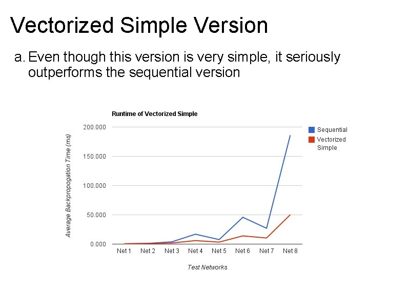
Vectorized Simple Version a. Even though this version is very simple, it seriously outperforms the sequential version

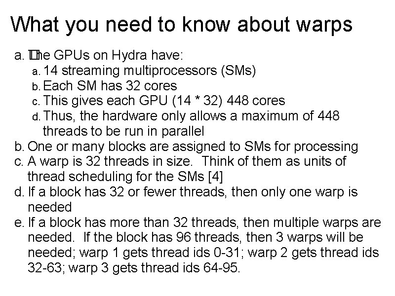
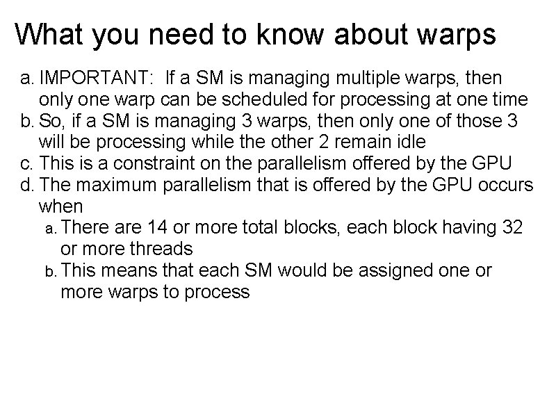
What you need to know about warps a. � The GPUs on Hydra have: a. 14 streaming multiprocessors (SMs) b. Each SM has 32 cores c. This gives each GPU (14 * 32) 448 cores d. Thus, the hardware only allows a maximum of 448 threads to be run in parallel b. One or many blocks are assigned to SMs for processing c. A warp is 32 threads in size. Think of them as units of thread scheduling for the SMs [4] d. If a block has 32 or fewer threads, then only one warp is needed e. If a block has more than 32 threads, then multiple warps are needed. If the block has 96 threads, then 3 warps will be needed; warp 1 gets thread ids 0 -31; warp 2 gets thread ids 32 -63; warp 3 gets thread ids 64 -95.

What you need to know about warps a. IMPORTANT: If a SM is managing multiple warps, then only one warp can be scheduled for processing at one time b. So, if a SM is managing 3 warps, then only one of those 3 will be processing while the other 2 remain idle c. This is a constraint on the parallelism offered by the GPU d. The maximum parallelism that is offered by the GPU occurs when a. There are 14 or more total blocks, each block having 32 or more threads b. This means that each SM would be assigned one or more warps to process

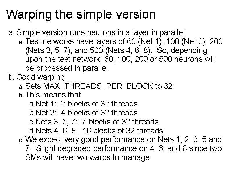
Warping the simple version a. Simple version runs neurons in a layer in parallel a. Test networks have layers of 60 (Net 1), 100 (Net 2), 200 (Nets 3, 5, 7), and 500 (Nets 4, 6, 8). So, depending upon the test network, 60, 100, 200 or 500 neurons will be processed in parallel b. Good warping a. Sets MAX_THREADS_PER_BLOCK to 32 b. This means that a. Net 1: 2 blocks of 32 threads b. Net 2: 4 blocks of 32 threads c. Nets 3, 5, 7: 7 blocks of 32 threads d. Nets 4, 6, 8: 16 blocks of 32 threads c. We expect very good performance on Nets 1, 2, 3, 5 and 7. Slight degraded performance on 4, 6, and 8 since two SMs will have two warps to manage

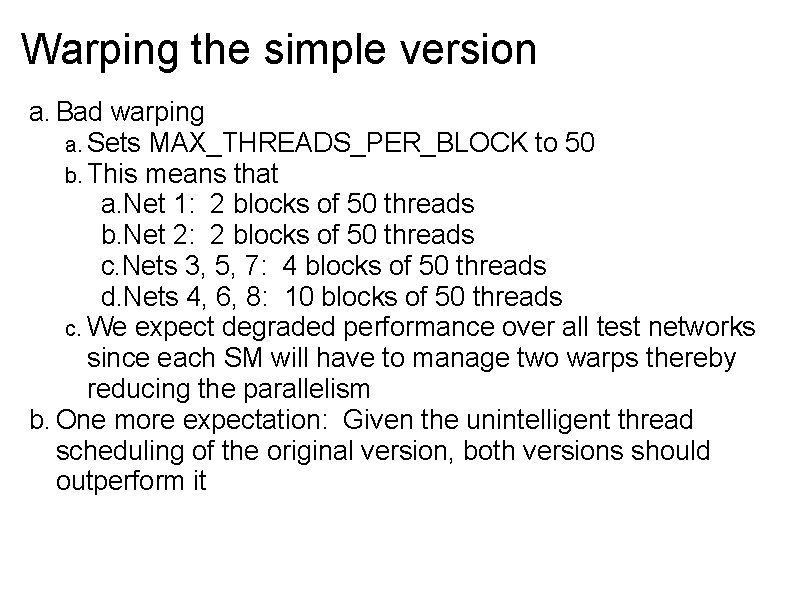
Warping the simple version a. Bad warping a. Sets MAX_THREADS_PER_BLOCK to 50 b. This means that a. Net 1: 2 blocks of 50 threads b. Net 2: 2 blocks of 50 threads c. Nets 3, 5, 7: 4 blocks of 50 threads d. Nets 4, 6, 8: 10 blocks of 50 threads c. We expect degraded performance over all test networks since each SM will have to manage two warps thereby reducing the parallelism b. One more expectation: Given the unintelligent thread scheduling of the original version, both versions should outperform it

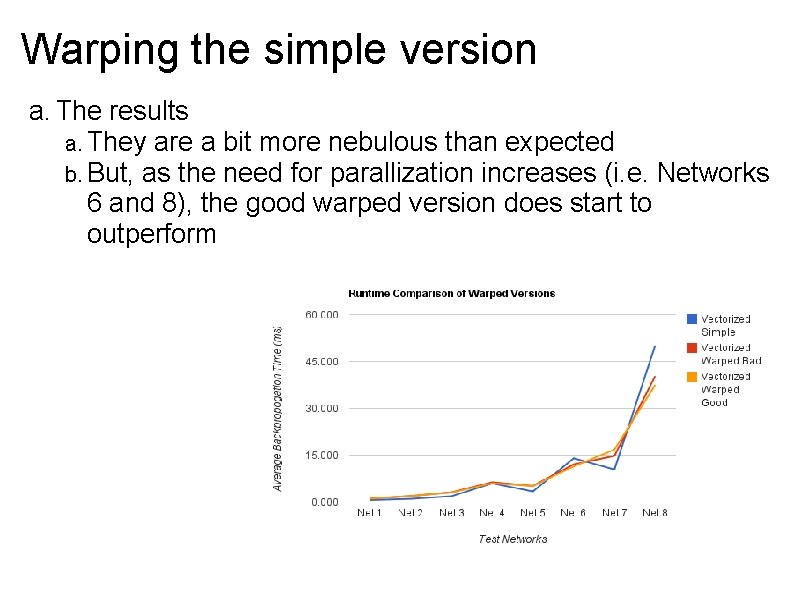
Warping the simple version a. The results a. They are a bit more nebulous than expected b. But, as the need for parallization increases (i. e. Networks 6 and 8), the good warped version does start to outperform

Puzzle Time a. So, why aren't the warped versions immediately faster than the simple version? E. g. the simple version is faster on Net 7 b. Some facts a. Each SM has L 1 and L 2 cache b. Threads within a warp have their memory reads grouped c. Memory that is close in locality to the areas being read are cached on the SM c. Technical information that I couldn't find a. Exact layout of global memory - When do we have collisions? b. Amount of data cached by an SM during a read - How often do the SMs have to go back to global memory? Nevertheless. . .

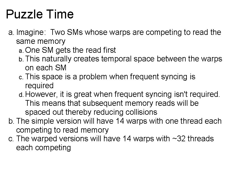
Puzzle Time a. Imagine: Two SMs whose warps are competing to read the same memory a. One SM gets the read first b. This naturally creates temporal space between the warps on each SM c. This space is a problem when frequent syncing is required d. However, it is great when frequent syncing isn't required. This means that subsequent memory reads will be spaced out thereby reducing collisions b. The simple version will have 14 warps with one thread each competing to read memory c. The warped versions will have 14 warps with ~32 threads each competing

Puzzle Time a. Ok. So why are warped versions slower on Net 7 and much faster on Net 8? b. Short answer: Density a. Density = ( neurons in a layer / actual concurrent threads) b. The more density, the more collisions c. If there is one thing to keep in mind when programming for the GPU, it is the notion of balance d. In this case, we are trying to balance the amount parallelism against the propensity for memory collisions e. The warped versions increase the concurrency and also increase the propensity for collisions (idleness) f. At some point, as the balance shifts, one affect or the other dominates

Puzzle Time a. Later, when we see the massively parallel version, we will see that having lots of warps per SM isn't necessarily a bad thing a. It can also mean that downstream warps benefit from cached data b. Again, back to balance : )

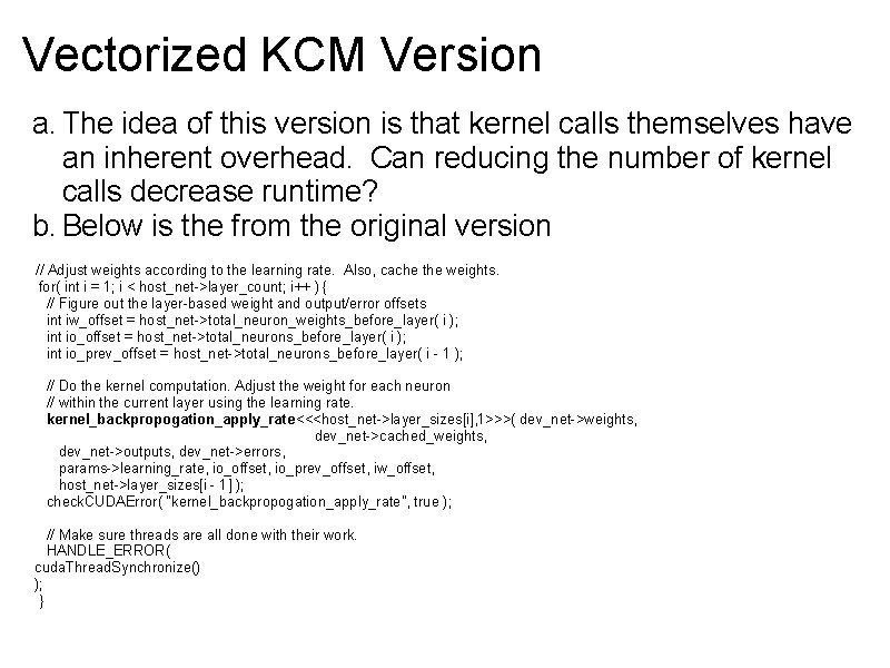
Vectorized KCM Version a. The idea of this version is that kernel calls themselves have an inherent overhead. Can reducing the number of kernel calls decrease runtime? b. Below is the from the original version // Adjust weights according to the learning rate. Also, cache the weights. for( int i = 1; i < host_net->layer_count; i++ ) { // Figure out the layer-based weight and output/error offsets int iw_offset = host_net->total_neuron_weights_before_layer( i ); int io_offset = host_net->total_neurons_before_layer( i ); int io_prev_offset = host_net->total_neurons_before_layer( i - 1 ); // Do the kernel computation. Adjust the weight for each neuron // within the current layer using the learning rate. kernel_backpropogation_apply_rate<<<host_net->layer_sizes[i], 1>>>( dev_net->weights, dev_net->cached_weights, dev_net->outputs, dev_net->errors, params->learning_rate, io_offset, io_prev_offset, iw_offset, host_net->layer_sizes[i - 1] ); check. CUDAError( "kernel_backpropogation_apply_rate", true ); // Make sure threads are all done with their work. HANDLE_ERROR( cuda. Thread. Synchronize() ); }

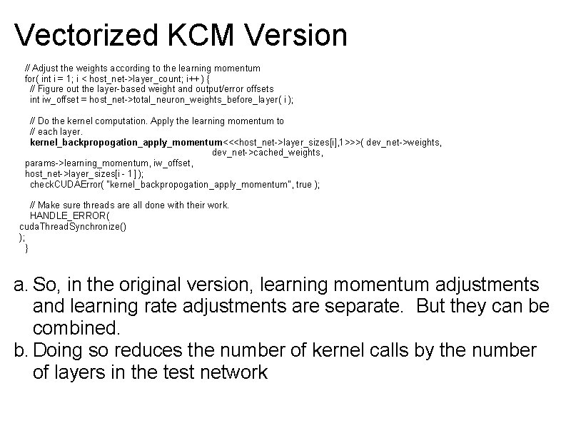
Vectorized KCM Version // Adjust the weights according to the learning momentum for( int i = 1; i < host_net->layer_count; i++ ) { // Figure out the layer-based weight and output/error offsets int iw_offset = host_net->total_neuron_weights_before_layer( i ); // Do the kernel computation. Apply the learning momentum to // each layer. kernel_backpropogation_apply_momentum<<<host_net->layer_sizes[i], 1>>>( dev_net->weights, dev_net->cached_weights, params->learning_momentum, iw_offset, host_net->layer_sizes[i - 1] ); check. CUDAError( "kernel_backpropogation_apply_momentum", true ); // Make sure threads are all done with their work. HANDLE_ERROR( cuda. Thread. Synchronize() ); } a. So, in the original version, learning momentum adjustments and learning rate adjustments are separate. But they can be combined. b. Doing so reduces the number of kernel calls by the number of layers in the test network

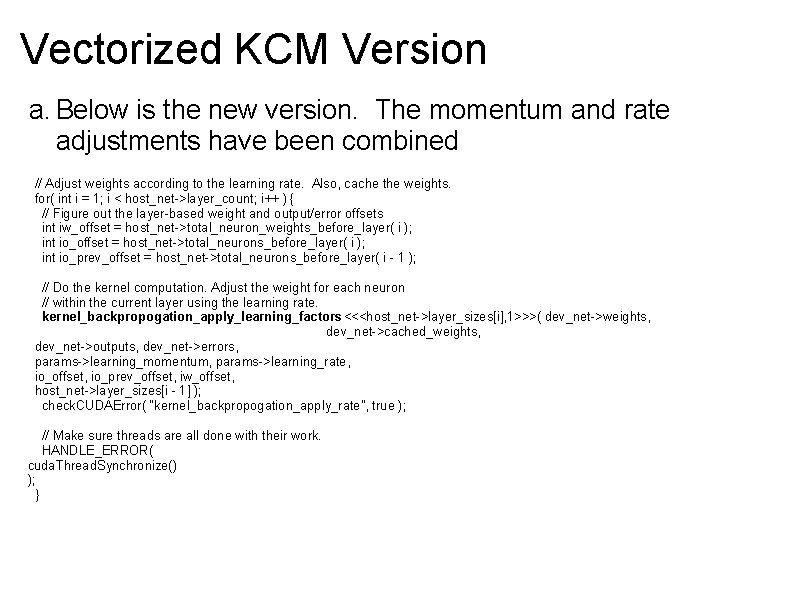
Vectorized KCM Version a. Below is the new version. The momentum and rate adjustments have been combined // Adjust weights according to the learning rate. Also, cache the weights. for( int i = 1; i < host_net->layer_count; i++ ) { // Figure out the layer-based weight and output/error offsets int iw_offset = host_net->total_neuron_weights_before_layer( i ); int io_offset = host_net->total_neurons_before_layer( i ); int io_prev_offset = host_net->total_neurons_before_layer( i - 1 ); // Do the kernel computation. Adjust the weight for each neuron // within the current layer using the learning rate. kernel_backpropogation_apply_learning_factors <<<host_net->layer_sizes[i], 1>>>( dev_net->weights, dev_net->cached_weights, dev_net->outputs, dev_net->errors, params->learning_momentum, params->learning_rate, io_offset, io_prev_offset, iw_offset, host_net->layer_sizes[i - 1] ); check. CUDAError( "kernel_backpropogation_apply_rate", true ); // Make sure threads are all done with their work. HANDLE_ERROR( cuda. Thread. Synchronize() ); }

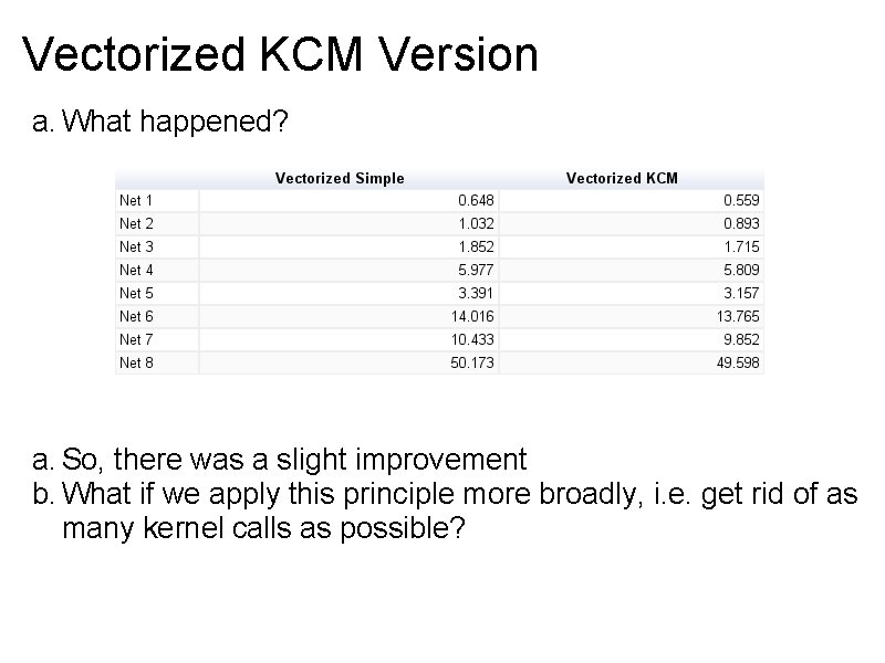
Vectorized KCM Version a. What happened? a. So, there was a slight improvement b. What if we apply this principle more broadly, i. e. get rid of as many kernel calls as possible?

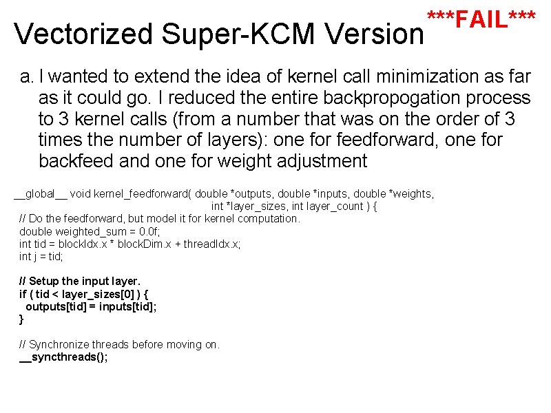
Vectorized Super-KCM Version ***FAIL*** a. I wanted to extend the idea of kernel call minimization as far as it could go. I reduced the entire backpropogation process to 3 kernel calls (from a number that was on the order of 3 times the number of layers): one for feedforward, one for backfeed and one for weight adjustment __global__ void kernel_feedforward( double *outputs, double *inputs, double *weights, int *layer_sizes, int layer_count ) { // Do the feedforward, but model it for kernel computation. double weighted_sum = 0. 0 f; int tid = block. Idx. x * block. Dim. x + thread. Idx. x; int j = tid; // Setup the input layer. if ( tid < layer_sizes[0] ) { outputs[tid] = inputs[tid]; } // Synchronize threads before moving on. __syncthreads();

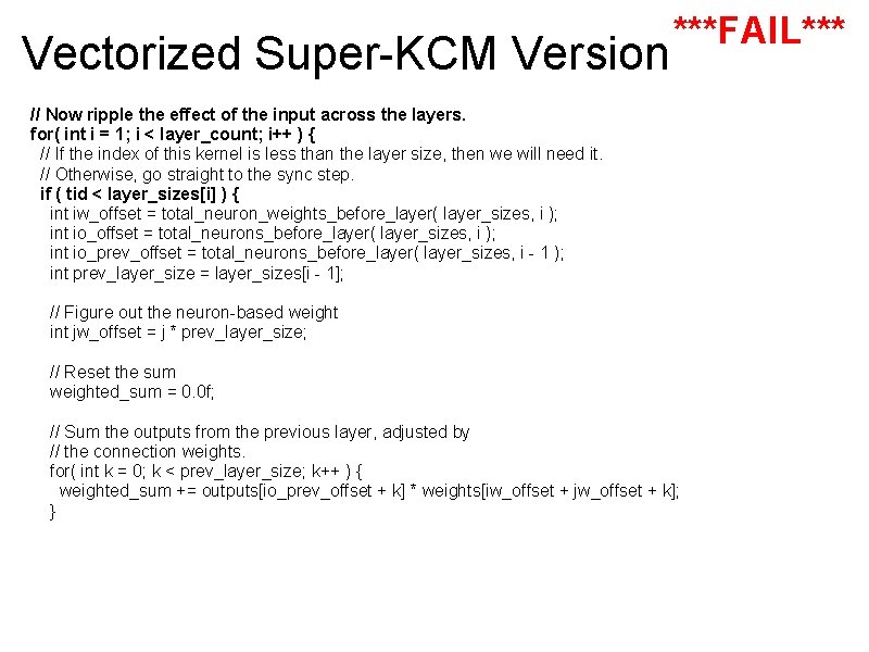
Vectorized Super-KCM Version ***FAIL*** // Now ripple the effect of the input across the layers. for( int i = 1; i < layer_count; i++ ) { // If the index of this kernel is less than the layer size, then we will need it. // Otherwise, go straight to the sync step. if ( tid < layer_sizes[i] ) { int iw_offset = total_neuron_weights_before_layer( layer_sizes, i ); int io_offset = total_neurons_before_layer( layer_sizes, i ); int io_prev_offset = total_neurons_before_layer( layer_sizes, i - 1 ); int prev_layer_size = layer_sizes[i - 1]; // Figure out the neuron-based weight int jw_offset = j * prev_layer_size; // Reset the sum weighted_sum = 0. 0 f; // Sum the outputs from the previous layer, adjusted by // the connection weights. for( int k = 0; k < prev_layer_size; k++ ) { weighted_sum += outputs[io_prev_offset + k] * weights[iw_offset + jw_offset + k]; }

Vectorized Super-KCM Version ***FAIL*** // Now, for this neuron, set the outputs[io_offset + j] = calculate_sigmoid( weighted_sum ); } // Synchronize threads before moving on. __syncthreads(); } a. This version didn't work. It failed because of the way that threads are synchonized b. The cuda procedure __syncthreads() is essentially a threadblock barrier. It ensures that all of the threads within a block have reached it before allowing any of them to move on c. The code that I wrote expected it to be a barrier for all threads within all blocks

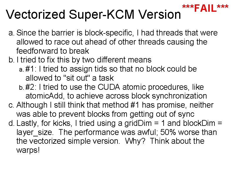
Vectorized Super-KCM Version ***FAIL*** a. Since the barrier is block-specific, I had threads that were allowed to race out ahead of other threads causing the feedforward to break b. I tried to fix this by two different means a. #1: I tried to assign tids so that no block could be allowed to "sit out" a task b. #2: I tried to use the CUDA atomic procedures, like atomic. Add, to achieve across block synchronization c. Although I still think that method #1 has promise, neither was able to prevent blocks from getting out of sync d. Lastly, for kicks, I tried using a grid. Dim = 1 and block. Dim = layer_size. The performance was awful; 50% worse than the vectorized simple version. Why? Think about the warps!

Vectorized Super-KCM Version ***FAIL*** a. Look at how bad this turned out a. So, the upshot is: Eliminate kernel calls where possible. However, be careful because they are the only way to achieve block-level synchronization b. Again, balance is in play. Balance between the cost of kernel calls and the need for global synchronization

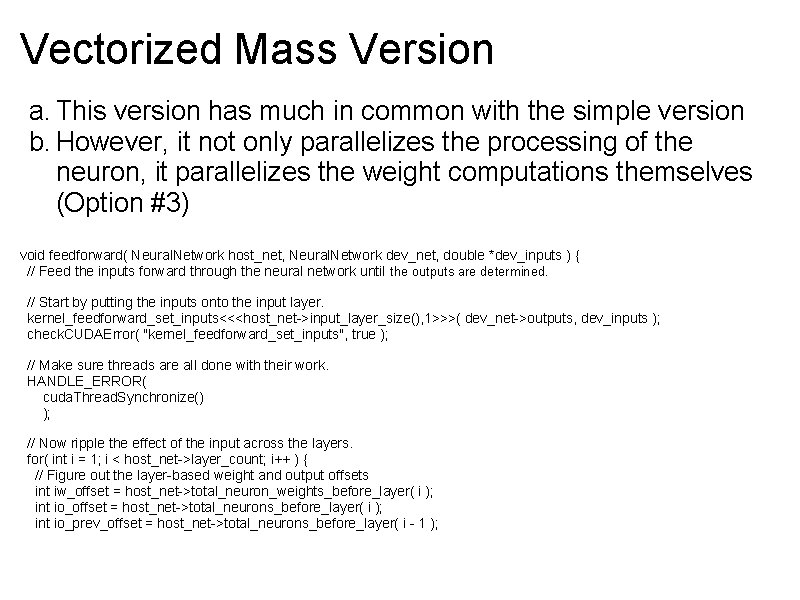
Vectorized Mass Version a. This version has much in common with the simple version b. However, it not only parallelizes the processing of the neuron, it parallelizes the weight computations themselves (Option #3) void feedforward( Neural. Network host_net, Neural. Network dev_net, double *dev_inputs ) { // Feed the inputs forward through the neural network until the outputs are determined. // Start by putting the inputs onto the input layer. kernel_feedforward_set_inputs<<<host_net->input_layer_size(), 1>>>( dev_net->outputs, dev_inputs ); check. CUDAError( "kernel_feedforward_set_inputs", true ); // Make sure threads are all done with their work. HANDLE_ERROR( cuda. Thread. Synchronize() ); // Now ripple the effect of the input across the layers. for( int i = 1; i < host_net->layer_count; i++ ) { // Figure out the layer-based weight and output offsets int iw_offset = host_net->total_neuron_weights_before_layer( i ); int io_offset = host_net->total_neurons_before_layer( i ); int io_prev_offset = host_net->total_neurons_before_layer( i - 1 );

Vectorized Mass Version // Do the kernel computation. kernel_feedforward<<<host_net->layer_sizes[i], host_net->layer_sizes[i - 1]>>>( dev_net->outputs, dev_net->weights, iw_offset, io_offset, io_prev_offset ); check. CUDAError( "kernel_feedforward", true ); // Make sure threads are all done with their work. HANDLE_ERROR( cuda. Thread. Synchronize() ); } } __global__ void kernel_feedforward( double *outputs, double *weights, int iw_offset, int io_prev_offset ) { // Do the feedforward, but model it for kernel computation. __shared__ double output_sums[512]; int prev_layer_size = block. Dim. x; int j = block. Idx. x; int k = thread. Idx. x; // Figure out the neuron-based weight int jw_offset = j * prev_layer_size; // Sum the outputs from the previous layer, adjusted by the connection weights. output_sums[k] = outputs[io_prev_offset + k] * weights[iw_offset + jw_offset + k];

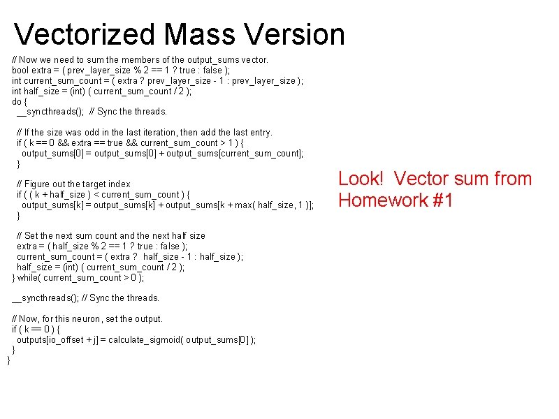
Vectorized Mass Version // Now we need to sum the members of the output_sums vector. bool extra = ( prev_layer_size % 2 == 1 ? true : false ); int current_sum_count = ( extra ? prev_layer_size - 1 : prev_layer_size ); int half_size = (int) ( current_sum_count / 2 ); do { __syncthreads(); // Sync the threads. // If the size was odd in the last iteration, then add the last entry. if ( k == 0 && extra == true && current_sum_count > 1 ) { output_sums[0] = output_sums[0] + output_sums[current_sum_count]; } // Figure out the target index if ( ( k + half_size ) < current_sum_count ) { output_sums[k] = output_sums[k] + output_sums[k + max( half_size, 1 )]; } // Set the next sum count and the next half size extra = ( half_size % 2 == 1 ? true : false ); current_sum_count = ( extra ? half_size - 1 : half_size ); half_size = (int) ( current_sum_count / 2 ); } while( current_sum_count > 0 ); __syncthreads(); // Sync the threads. // Now, for this neuron, set the output. if ( k == 0 ) { outputs[io_offset + j] = calculate_sigmoid( output_sums[0] ); } } Look! Vector sum from Homework #1

Vectorized Mass Version a. So, the kernel call dimensions blocks according to the number of neurons in the current layer; the number of threads according to the number of neurons in the previous layer b. Each thread calculates its respective weight value c. All of the threads within each block then do a vector-sum in order to determine the output. This should look very familiar. I designed it based upon our first homework assignment d. So, how does it perform?

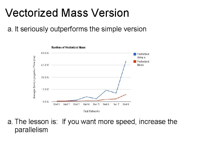
Vectorized Mass Version a. It seriously outperforms the simple version a. The lesson is: If you want more speed, increase the parallelism

Vectorized Mass Version a. One more quick note a. When processing Net 8, each SM is saddled with ~550 warps. Wow! b. Yet, we know that only 14 of these can be processed at once (448 concurrent threads) c. Where is speed? d. In this case, there is a benefit from lots of warps per SM. They are benefiting from the L 1 and L 2 caches on each SM e. In the global memory fetches per thread is much lower for this version. Yay!

Vectorized KCM Mass Version a. This version is the Vectorized Mass version, except, during backpropogation, the weight adjustments have been combined (like the Vectorized KCM) version b. What happens? Again, kernel call minimization yields modest benefits

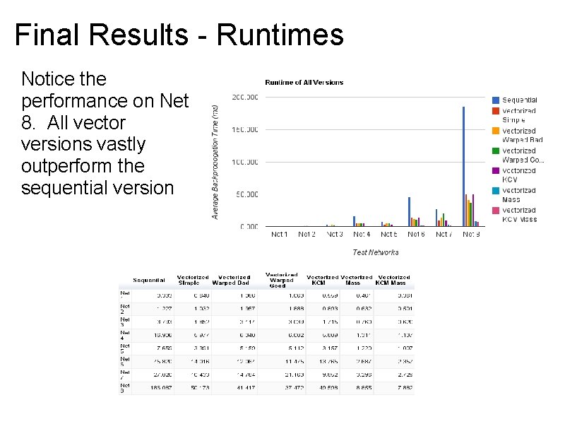
Final Results - Runtimes Notice the performance on Net 8. All vector versions vastly outperform the sequential version

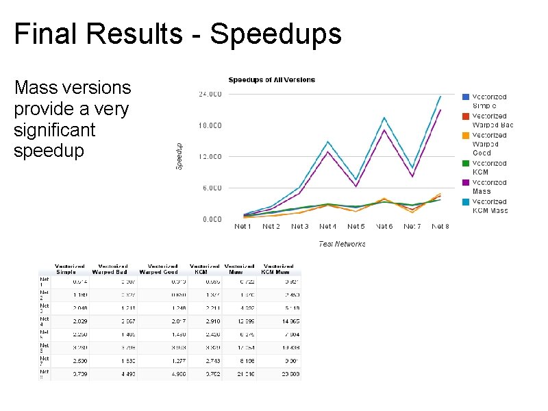
Final Results - Speedups Mass versions provide a very significant speedup

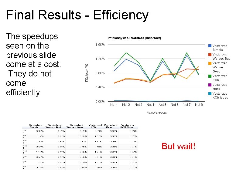
Final Results - Efficiency The speedups seen on the previous slide come at a cost. They do not come efficiently But wait!

Wait! Given what we know of warps, let's rethink efficiency a. The efficiency data on the previous slide was based on the number concurrent threads. However, based on what we have learned about warps, we know that the number of actual concurrent threads can be no more than 448. Given that the Vectorized Mass version uses 250, 000 concurrent threads, this realization will make a huge difference in the efficiency numbers b. So, let's go back and figure out the number cores used for the various networks

Real Efficiency a. Vectorized Simple a. Dimensions blocks only so each thread is alone within its warp b. Erroneously assumed that all neurons were processing at once so it assumed number of cores to be 200 -500, depending on the test network c. Therefore, no more than 14 cores are processing at one time b. Vectorized Warped Good a. Attempts to dimension so that all cores are occupied b. So, if the maximum layer size of the test network is 200, then 200 cores are processing at once; if it is 500, then all 448 cores are processing at once

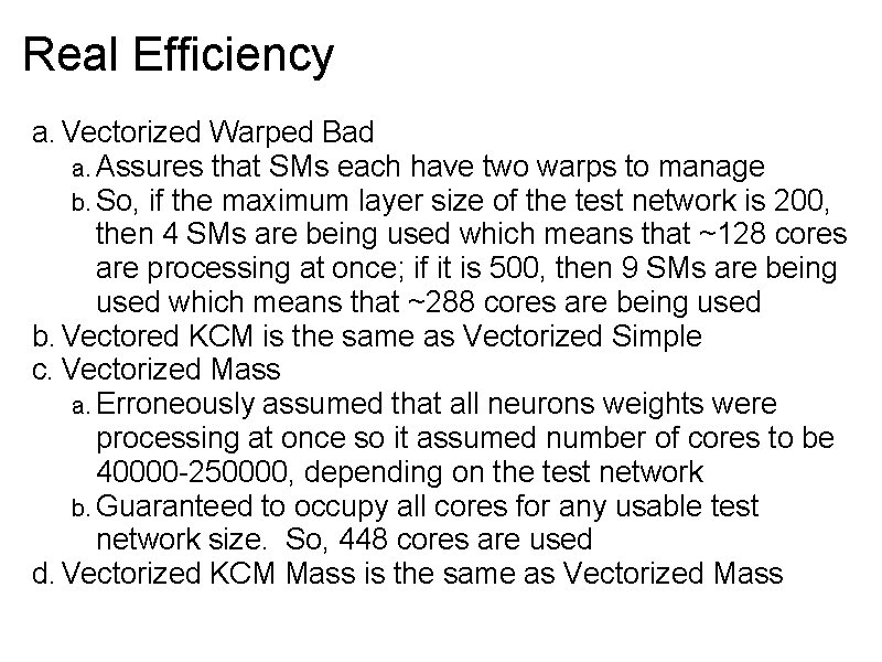
Real Efficiency a. Vectorized Warped Bad a. Assures that SMs each have two warps to manage b. So, if the maximum layer size of the test network is 200, then 4 SMs are being used which means that ~128 cores are processing at once; if it is 500, then 9 SMs are being used which means that ~288 cores are being used b. Vectored KCM is the same as Vectorized Simple c. Vectorized Mass a. Erroneously assumed that all neurons weights were processing at once so it assumed number of cores to be 40000 -250000, depending on the test network b. Guaranteed to occupy all cores for any usable test network size. So, 448 cores are used d. Vectorized KCM Mass is the same as Vectorized Mass

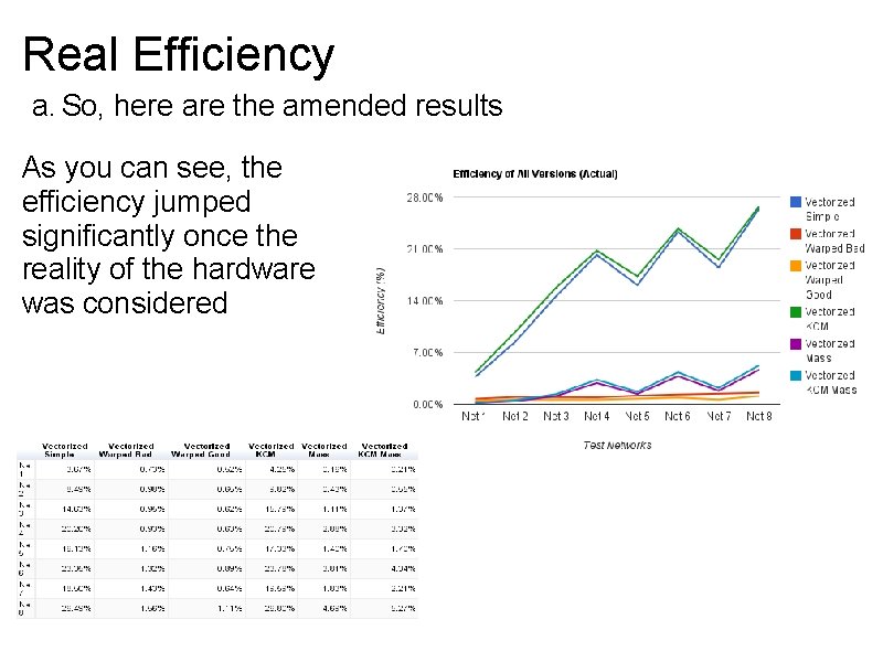
Real Efficiency a. So, here are the amended results As you can see, the efficiency jumped significantly once the reality of the hardware was considered

Why is efficiency less than one? a. So, I think it is always worth asking: why was my efficiency less than 1? a. In other words, if I use 10 CPUs to tackle a problem, why didn't I get a 10 times speedup? b. Reasons for efficiency a. The efficiency calculation is based upon the width of the largest layer, since this will be the highest number of SM cores used during the process b. Neither feedforward nor backpropogation are globally parallel. Remember the KCM Fail version c. As we've seen, warps can be idle on an SM when they are swapped out d. Warps can be idle while the SM cache is being populated with the outputs from the previous layer

Future Thoughts a. Just for fun, I'd love to train a neural network to break substitution ciphers a. The neural network would need to be very large a. The input layer, by itself, would need to be between 7 * 500 and 7 * 2000 in size to be remotely useful b. Therefore, the vectorized neural network algorithm would need to be heavily strip mined a. Thereby, decreasing speedup (but raising overall efficiency) c. Or. . a. The network processing could be distributed across multiple GPUs using Open. MP or MPI d. I think that the basic tools for doing so are already in there

Conclusions a. GPU-based hardware can be used to gain significant speedups when processing neural networks b. While CUDA provides lots of different mechanisms for interacting with the GPU, one must start with a thorough understanding the hardware, e. g. how it can be synchronized, how its threads are managed, etc c. More is more - More parallelism can boost performance d. The bottom line is: Start with the basic hardware! Before reading about all of the special methods, start by understanding how the basic ones are actually implemented

References