Parallel Prefix Pack and Sorting Outline Done Simple

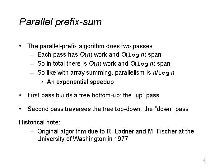
Parallel Prefix, Pack, and Sorting

Outline Done: – Simple ways to use parallelism for counting, summing, finding – Analysis of running time and implications of Amdahl’s Law Now: Clever ways to parallelize more than is intuitively possible – Parallel prefix: • This “key trick” typically underlies surprising parallelization • Enables other things like packs – Parallel sorting: quicksort (not in place) and mergesort • Easy to get a little parallelism • With cleverness can get a lot 2

The prefix-sum problem Given int[] input, produce int[] output where output[i] is the sum of input[0]+input[1]+…+input[i] Sequential can be a CS 1 exam problem: int[] prefix_sum(int[] input){ int[] output = new int[input. length]; output[0] = input[0]; for(int i=1; i < input. length; i++) output[i] = output[i-1]+input[i]; return output; } Does not seem parallelizable – Work: O(n), Span: O(n) – This algorithm is sequential, but a different algorithm has Work: O(n), Span: O(log n) 3

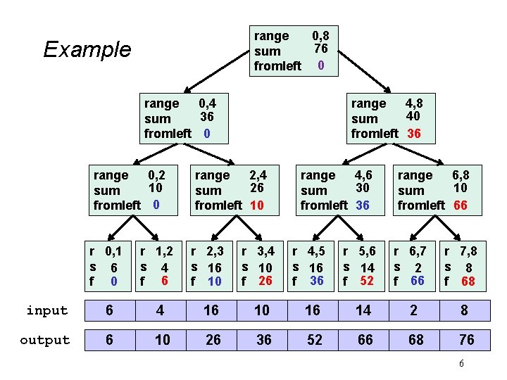
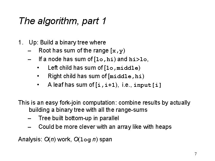
Parallel prefix-sum • The parallel-prefix algorithm does two passes – Each pass has O(n) work and O(log n) span – So in total there is O(n) work and O(log n) span – So like with array summing, parallelism is n/log n • An exponential speedup • First pass builds a tree bottom-up: the “up” pass • Second pass traverses the tree top-down: the “down” pass Historical note: – Original algorithm due to R. Ladner and M. Fischer at the University of Washington in 1977 4

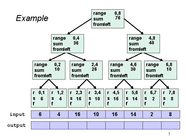
range 0, 8 76 sum fromleft Example range 0, 4 36 sum fromleft range 0, 2 10 sum fromleft input range 4, 8 40 sum fromleft range 2, 4 26 sum fromleft range 4, 6 30 sum fromleft range 6, 8 10 sum fromleft r 0, 1 s 6 f r 1, 2 s 4 f r 2, 3 s 16 f r 3, 4 s 10 f r 4, 5 s 16 f r 5, 6 s 14 f r 6, 7 s 2 f r 7, 8 s 8 f 6 4 16 10 16 14 2 8 output 5

range 0, 8 76 sum fromleft 0 Example range 0, 4 36 sum fromleft 0 range 0, 2 10 sum fromleft 0 range 4, 8 40 sum fromleft 36 range 2, 4 26 sum fromleft 10 range 4, 6 30 sum fromleft 36 range 6, 8 10 sum fromleft 66 r 0, 1 s 6 f 0 r 1, 2 s 4 f 6 r 2, 3 s 16 f 10 r 3, 4 s 10 f 26 r 4, 5 s 16 f 36 r 5, 6 s 14 f 52 r 6, 7 s 2 f 66 r 7, 8 s 8 f 68 input 6 4 16 10 16 14 2 8 output 6 10 26 36 52 66 68 76 6

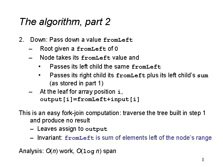
The algorithm, part 1 1. Up: Build a binary tree where – Root has sum of the range [x, y) – If a node has sum of [lo, hi) and hi>lo, • Left child has sum of [lo, middle) • Right child has sum of [middle, hi) • A leaf has sum of [i, i+1), i. e. , input[i] This is an easy fork-join computation: combine results by actually building a binary tree with all the range-sums – Tree built bottom-up in parallel – Could be more clever with an array like with heaps Analysis: O(n) work, O(log n) span 7

The algorithm, part 2 2. Down: Pass down a value from. Left – Root given a from. Left of 0 – Node takes its from. Left value and • Passes its left child the same from. Left • Passes its right child its from. Left plus its left child’s sum (as stored in part 1) – At the leaf for array position i, output[i]=from. Left+input[i] This is an easy fork-join computation: traverse the tree built in step 1 and produce no result – Leaves assign to output – Invariant: from. Left is sum of elements left of the node’s range Analysis: O(n) work, O(log n) span 8

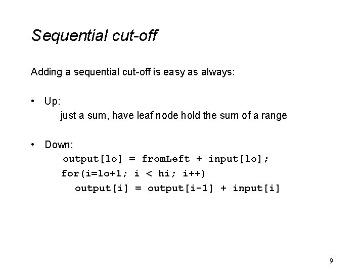
Sequential cut-off Adding a sequential cut-off is easy as always: • Up: just a sum, have leaf node hold the sum of a range • Down: output[lo] = from. Left + input[lo]; for(i=lo+1; i < hi; i++) output[i] = output[i-1] + input[i] 9

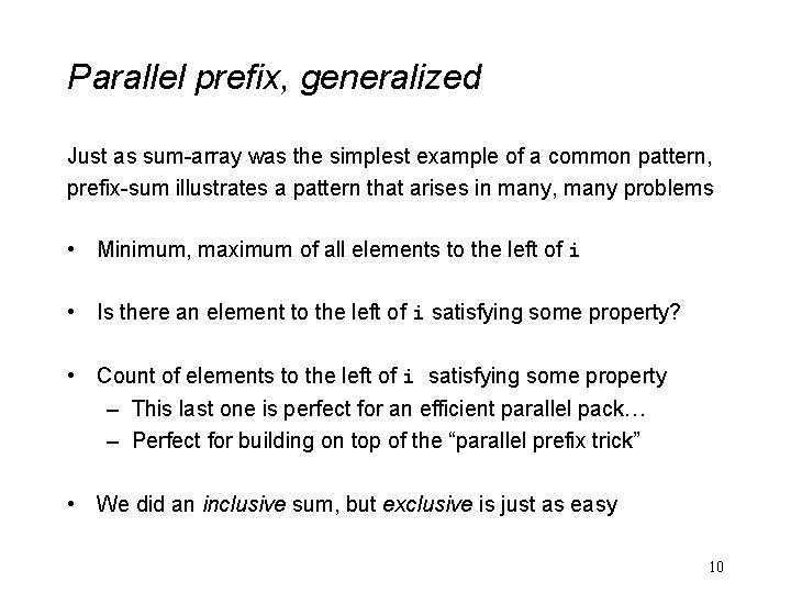
Parallel prefix, generalized Just as sum-array was the simplest example of a common pattern, prefix-sum illustrates a pattern that arises in many, many problems • Minimum, maximum of all elements to the left of i • Is there an element to the left of i satisfying some property? • Count of elements to the left of i satisfying some property – This last one is perfect for an efficient parallel pack… – Perfect for building on top of the “parallel prefix trick” • We did an inclusive sum, but exclusive is just as easy 10

Pack [Non-standard terminology] Given an array input, produce an array output containing only elements such that f(elt) is true Example: input [17, 4, 6, 8, 11, 5, 13, 19, 0, 24] f: is elt > 10 output [17, 11, 13, 19, 24] Parallelizable? – Finding elements for the output is easy – But getting them in the right place seems hard 11

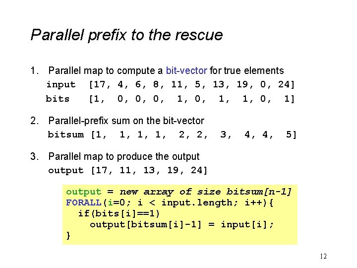
Parallel prefix to the rescue 1. Parallel map to compute a bit-vector for true elements input [17, 4, 6, 8, 11, 5, 13, 19, 0, 24] bits [1, 0, 0, 0, 1, 1, 0, 1] 2. Parallel-prefix sum on the bit-vector bitsum [1, 1, 2, 2, 3, 4, 4, 5] 3. Parallel map to produce the output [17, 11, 13, 19, 24] output = new array of size bitsum[n-1] FORALL(i=0; i < input. length; i++){ if(bits[i]==1) output[bitsum[i]-1] = input[i]; } 12

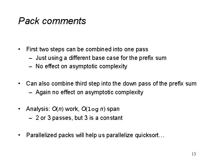
Pack comments • First two steps can be combined into one pass – Just using a different base case for the prefix sum – No effect on asymptotic complexity • Can also combine third step into the down pass of the prefix sum – Again no effect on asymptotic complexity • Analysis: O(n) work, O(log n) span – 2 or 3 passes, but 3 is a constant • Parallelized packs will help us parallelize quicksort… 13

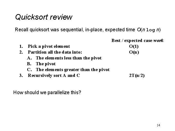
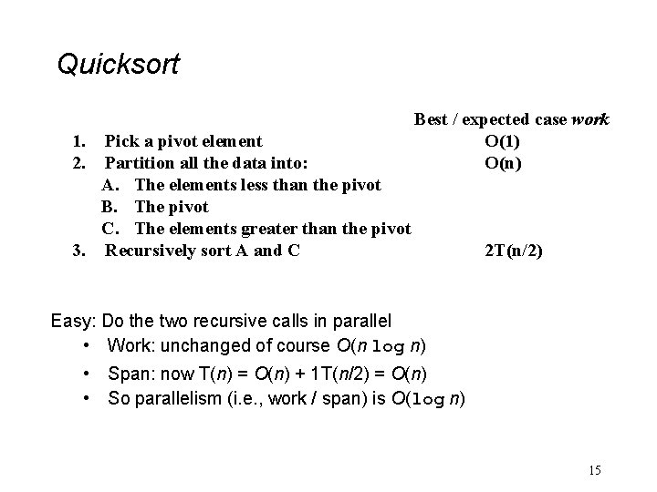
Quicksort review Recall quicksort was sequential, in-place, expected time O(n log n) 1. 2. Pick a pivot element Partition all the data into: A. The elements less than the pivot B. The pivot C. The elements greater than the pivot 3. Recursively sort A and C Best / expected case work O(1) O(n) 2 T(n/2) How should we parallelize this? 14

Quicksort 1. 2. Pick a pivot element Partition all the data into: A. The elements less than the pivot B. The pivot C. The elements greater than the pivot 3. Recursively sort A and C Best / expected case work O(1) O(n) 2 T(n/2) Easy: Do the two recursive calls in parallel • Work: unchanged of course O(n log n) • Span: now T(n) = O(n) + 1 T(n/2) = O(n) • So parallelism (i. e. , work / span) is O(log n) 15

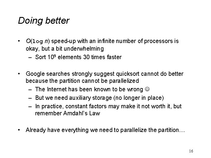
Doing better • O(log n) speed-up with an infinite number of processors is okay, but a bit underwhelming – Sort 109 elements 30 times faster • Google searches strongly suggest quicksort cannot do better because the partition cannot be parallelized – The Internet has been known to be wrong – But we need auxiliary storage (no longer in place) – In practice, constant factors may make it not worth it, but remember Amdahl’s Law • Already have everything we need to parallelize the partition… 16

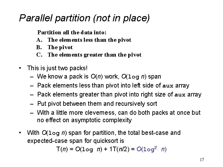
Parallel partition (not in place) Partition all the data into: A. The elements less than the pivot B. The pivot C. The elements greater than the pivot • This is just two packs! – We know a pack is O(n) work, O(log n) span – Pack elements less than pivot into left side of aux array – Pack elements greater than pivot into right size of aux array – Put pivot between them and recursively sort – With a little more cleverness, can do both packs at once but no effect on asymptotic complexity • With O(log n) span for partition, the total best-case and expected-case span for quicksort is T(n) = O(log n) + 1 T(n/2) = O(log 2 n) 17

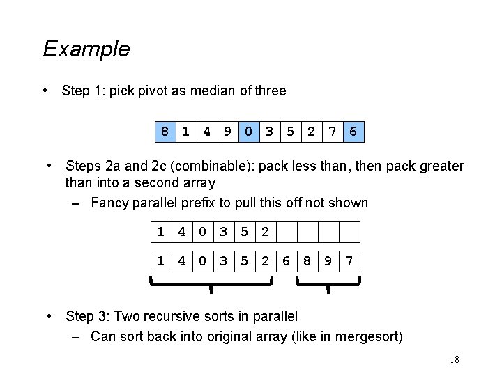
Example • Step 1: pick pivot as median of three 8 1 4 9 0 3 5 2 7 6 • Steps 2 a and 2 c (combinable): pack less than, then pack greater than into a second array – Fancy parallel prefix to pull this off not shown 1 4 0 3 5 2 6 8 9 7 • Step 3: Two recursive sorts in parallel – Can sort back into original array (like in mergesort) 18

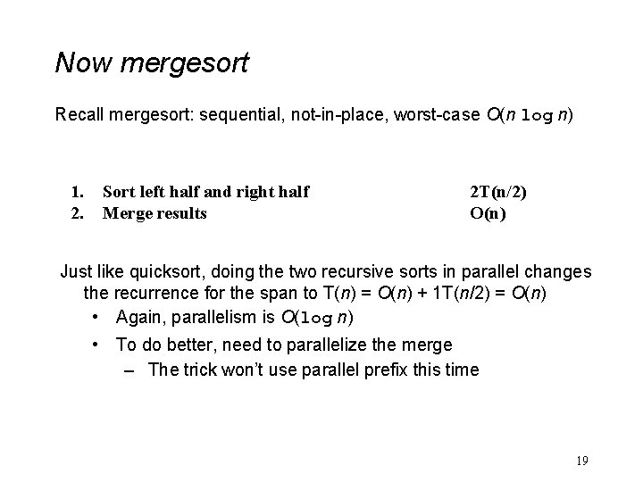
Now mergesort Recall mergesort: sequential, not-in-place, worst-case O(n log n) 1. 2. Sort left half and right half Merge results 2 T(n/2) O(n) Just like quicksort, doing the two recursive sorts in parallel changes the recurrence for the span to T(n) = O(n) + 1 T(n/2) = O(n) • Again, parallelism is O(log n) • To do better, need to parallelize the merge – The trick won’t use parallel prefix this time 19

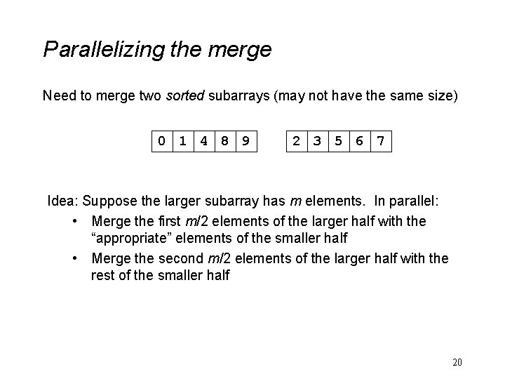
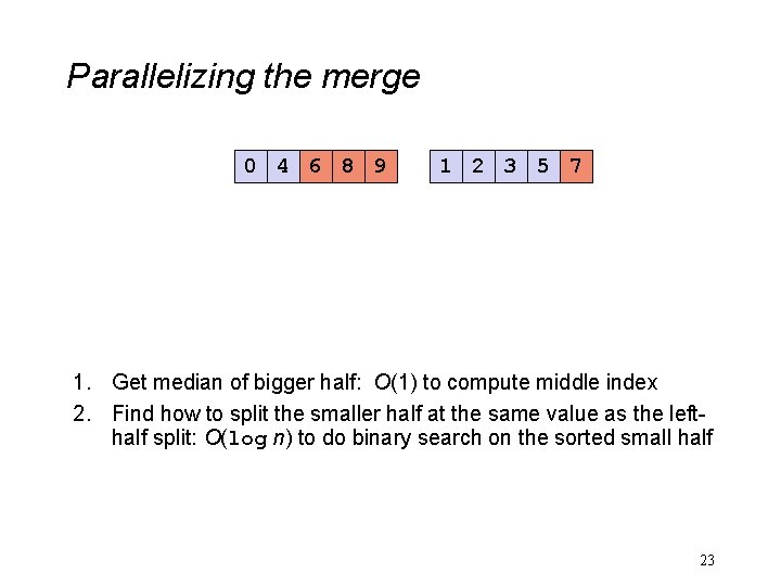
Parallelizing the merge Need to merge two sorted subarrays (may not have the same size) 0 1 4 8 9 2 3 5 6 7 Idea: Suppose the larger subarray has m elements. In parallel: • Merge the first m/2 elements of the larger half with the “appropriate” elements of the smaller half • Merge the second m/2 elements of the larger half with the rest of the smaller half 20

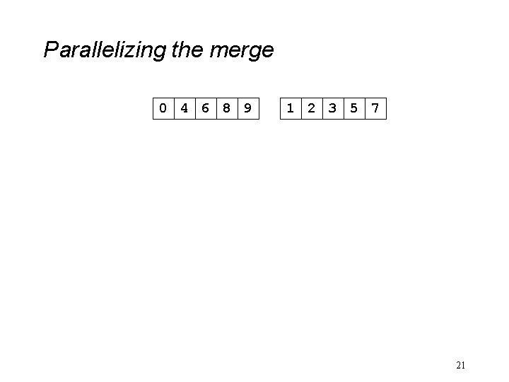
Parallelizing the merge 0 4 6 8 9 1 2 3 5 7 21

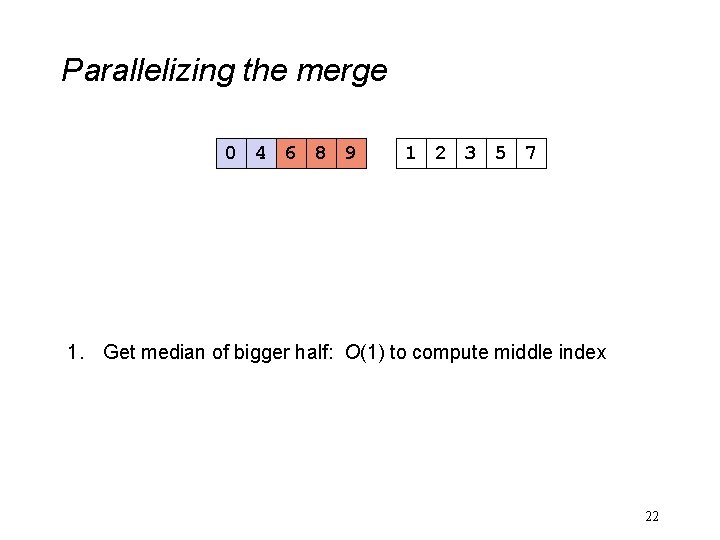
Parallelizing the merge 0 4 6 8 9 1 2 3 5 7 1. Get median of bigger half: O(1) to compute middle index 22

Parallelizing the merge 0 4 6 8 9 1 2 3 5 7 1. Get median of bigger half: O(1) to compute middle index 2. Find how to split the smaller half at the same value as the lefthalf split: O(log n) to do binary search on the sorted small half 23

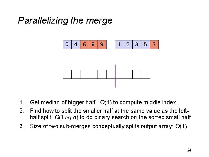
Parallelizing the merge 0 4 6 8 9 1 2 3 5 7 1. Get median of bigger half: O(1) to compute middle index 2. Find how to split the smaller half at the same value as the lefthalf split: O(log n) to do binary search on the sorted small half 3. Size of two sub-merges conceptually splits output array: O(1) 24

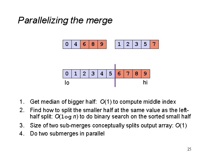
Parallelizing the merge 0 4 6 8 9 1 2 3 5 7 0 1 2 3 4 5 6 7 8 9 lo hi 1. Get median of bigger half: O(1) to compute middle index 2. Find how to split the smaller half at the same value as the lefthalf split: O(log n) to do binary search on the sorted small half 3. Size of two sub-merges conceptually splits output array: O(1) 4. Do two submerges in parallel 25

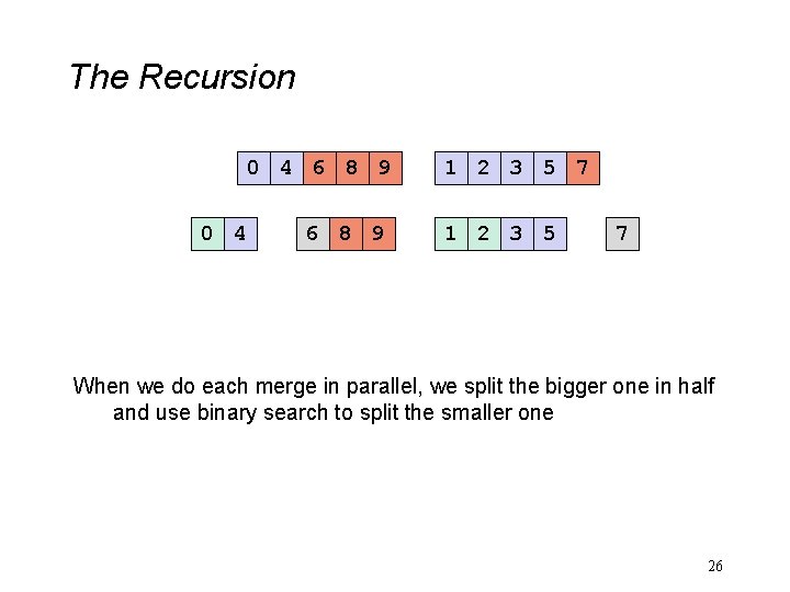
The Recursion 0 4 6 8 9 1 2 3 5 7 When we do each merge in parallel, we split the bigger one in half and use binary search to split the smaller one 26

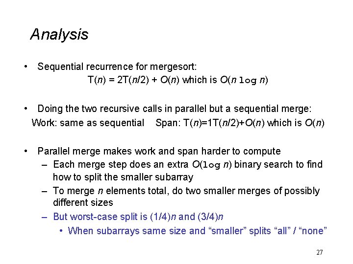
Analysis • Sequential recurrence for mergesort: T(n) = 2 T(n/2) + O(n) which is O(n log n) • Doing the two recursive calls in parallel but a sequential merge: Work: same as sequential Span: T(n)=1 T(n/2)+O(n) which is O(n) • Parallel merge makes work and span harder to compute – Each merge step does an extra O(log n) binary search to find how to split the smaller subarray – To merge n elements total, do two smaller merges of possibly different sizes – But worst-case split is (1/4)n and (3/4)n • When subarrays same size and “smaller” splits “all” / “none” 27

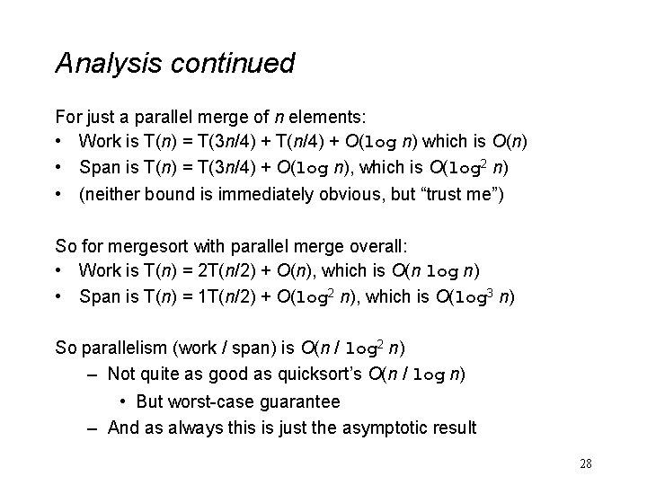
Analysis continued For just a parallel merge of n elements: • Work is T(n) = T(3 n/4) + T(n/4) + O(log n) which is O(n) • Span is T(n) = T(3 n/4) + O(log n), which is O(log 2 n) • (neither bound is immediately obvious, but “trust me”) So for mergesort with parallel merge overall: • Work is T(n) = 2 T(n/2) + O(n), which is O(n log n) • Span is T(n) = 1 T(n/2) + O(log 2 n), which is O(log 3 n) So parallelism (work / span) is O(n / log 2 n) – Not quite as good as quicksort’s O(n / log n) • But worst-case guarantee – And as always this is just the asymptotic result 28