Parallel Paradigms and Examples Topics n Data Parallelism

Parallel Paradigms and Examples Topics n Data Parallelism Pipelines Task Queues n Examples n n

Previously Ordering of statements. Dependences. Parallelism. Synchronization. – 2–

Goal of next few lectures Standard patterns of parallel programs. Examples of each. Later, code examples in various programming models. – 3–

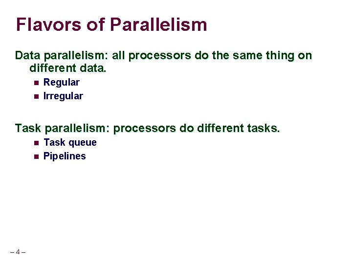
Flavors of Parallelism Data parallelism: all processors do the same thing on different data. n n Regular Irregular Task parallelism: processors do different tasks. n n – 4– Task queue Pipelines

Data Parallelism Essential idea: each processor works on a different part of the data (usually in one or more arrays). Regular or irregular data parallelism: using linear or non-linear indexing. Examples: MM (regular), SOR (regular), MD (irregular). – 5–

Matrix Multiplication of two n by n matrices A and B into a third n by n matrix C – 6–

Matrix Multiply for( i=0; i<n; i++ ) for( j=0; j<n; j++ ) c[i][j] = 0. 0; for( i=0; i<n; i++ ) for( j=0; j<n; j++ ) for( k=0; k<n; k++ ) c[i][j] += a[i][k]*b[k][j]; – 7–

Parallel Matrix Multiply No loop-carried dependences in i- or j-loop. Loop-carried dependence on k-loop. All i- and j-iterations can be run in parallel. – 8–

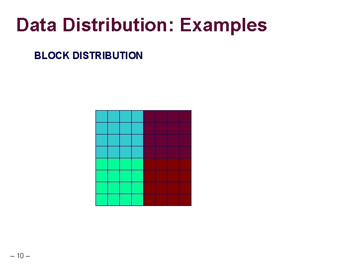
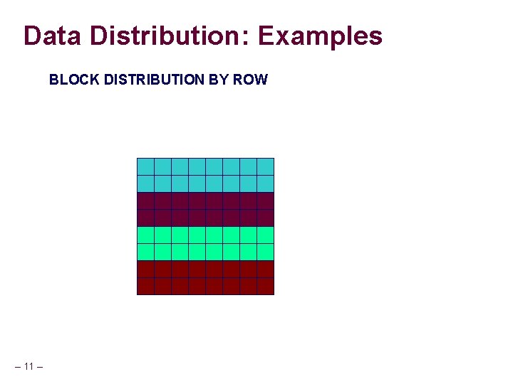
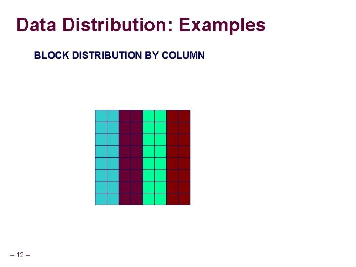
Parallel Matrix Multiply (contd. ) If we have P processors, we can give n/P rows or columns to each processor. Or, we can divide the matrix in P squares, and give each processor one square. – 9–

Data Distribution: Examples BLOCK DISTRIBUTION – 10 –

Data Distribution: Examples BLOCK DISTRIBUTION BY ROW – 11 –

Data Distribution: Examples BLOCK DISTRIBUTION BY COLUMN – 12 –

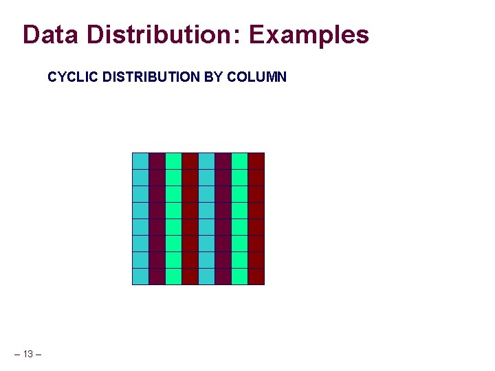
Data Distribution: Examples CYCLIC DISTRIBUTION BY COLUMN – 13 –

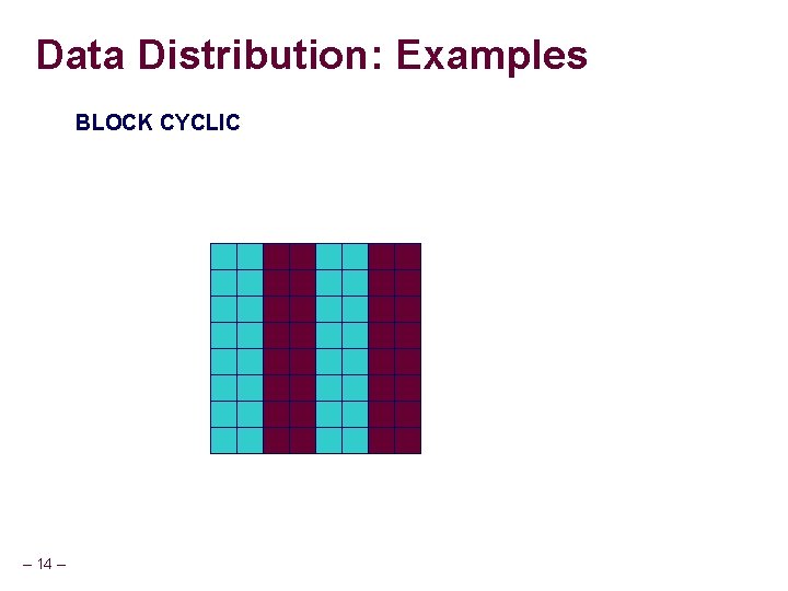
Data Distribution: Examples BLOCK CYCLIC – 14 –

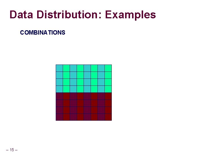
Data Distribution: Examples COMBINATIONS – 15 –

Task Parallelism Each process performs a different task. Two principal flavors: n n pipelines task queues Program Examples: PIPE (pipeline), TSP (task queue). – 16 –

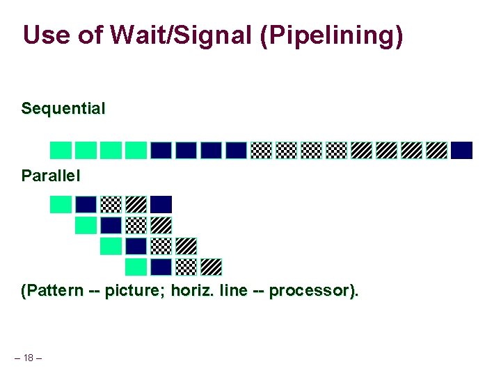
Pipeline Often occurs with image processing applications, where a number of images undergoes a sequence of transformations. E. g. , rendering, clipping, compression, etc. – 17 –

Use of Wait/Signal (Pipelining) Sequential Parallel (Pattern -- picture; horiz. line -- processor). – 18 –

PIPE P 1: for( i=0; i<num_pics, read(in_pic); i++ ) { int_pic_1[i] = trans 1( in_pic ); signal( event_1_2[i] ); } P 2: for( i=0; i<num_pics; i++ ) { wait( event_1_2[i] ); int_pic_2[i] = trans 2( int_pic_1[i] ); signal( event_2_3[i] ); } – 19 –

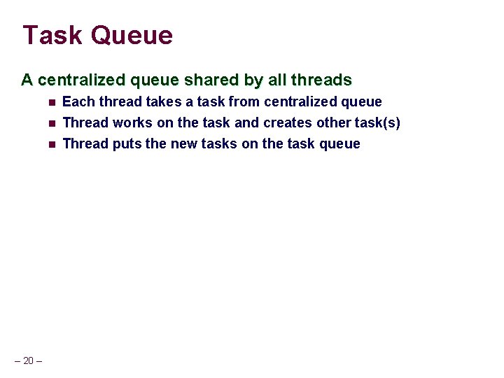
Task Queue A centralized queue shared by all threads n Each thread takes a task from centralized queue n Thread works on the task and creates other task(s) Thread puts the new tasks on the task queue n – 20 –

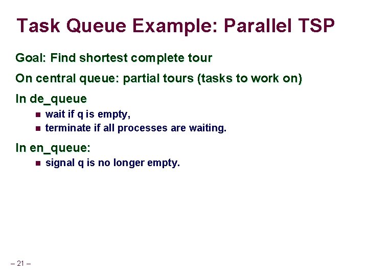
Task Queue Example: Parallel TSP Goal: Find shortest complete tour On central queue: partial tours (tasks to work on) In de_queue n n wait if q is empty, terminate if all processes are waiting. In en_queue: n – 21 – signal q is no longer empty.

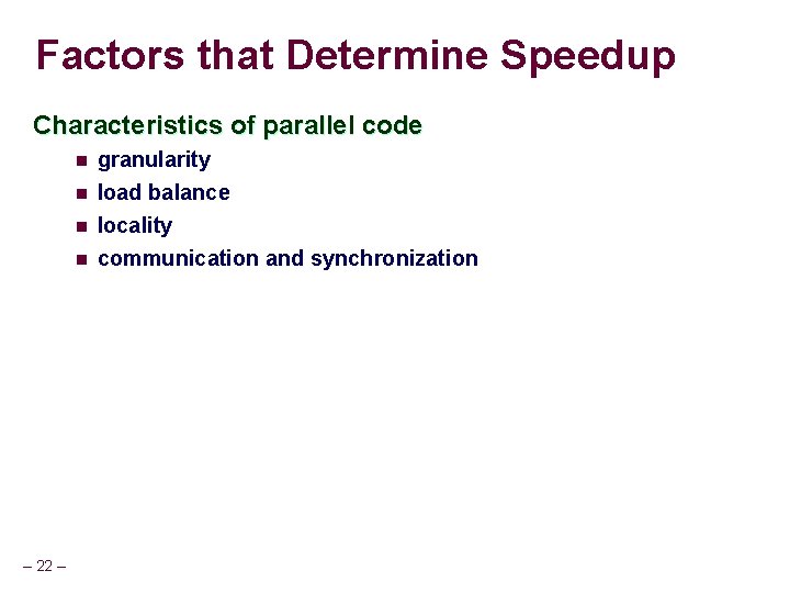
Factors that Determine Speedup Characteristics of parallel code n granularity n load balance locality communication and synchronization n n – 22 –

Granularity = size of the program unit that is executed by a single processor. May be a single loop iteration, a set of loop iterations, etc. Fine granularity leads to: n (positive) ability to use lots of processors n (positive) finer-grain load balancing n (negative) increased overhead – 23 –

Granularity and Critical Sections Small granularity => more processors => more critical section accesses => more contention. – 24 –

Issues in Performance of Parallel Parts Granularity. Load balance. Locality. Synchronization and communication. – 25 –

Load Balance Load imbalance = different in execution time between processors between barriers. Execution time may not be predictable. n n n – 26 – Regular data parallel: yes. Irregular data parallel or pipeline: perhaps. Task queue: no.

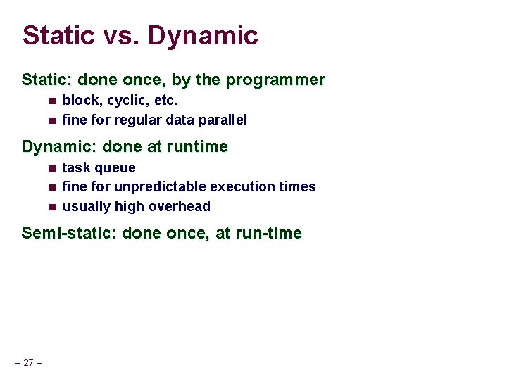
Static vs. Dynamic Static: done once, by the programmer n n block, cyclic, etc. fine for regular data parallel Dynamic: done at runtime n n n task queue fine for unpredictable execution times usually high overhead Semi-static: done once, at run-time – 27 –

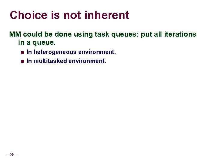
Choice is not inherent MM could be done using task queues: put all iterations in a queue. n n – 28 – In heterogeneous environment. In multitasked environment.

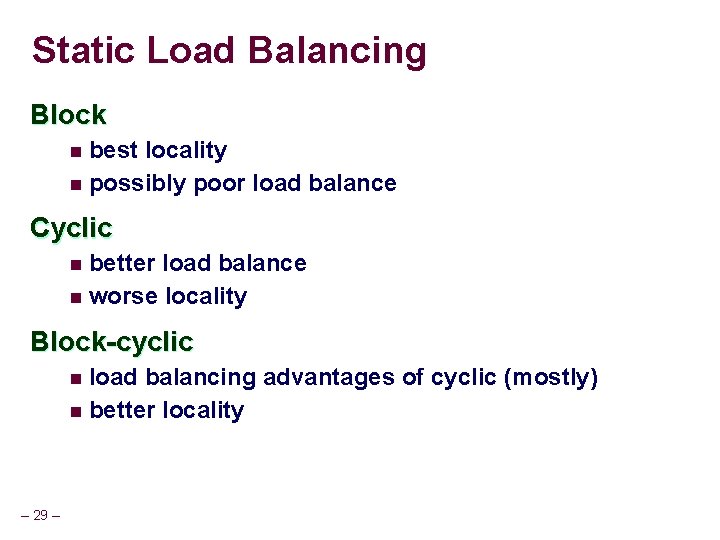
Static Load Balancing Block best locality n possibly poor load balance n Cyclic better load balance n worse locality n Block-cyclic load balancing advantages of cyclic (mostly) n better locality n – 29 –

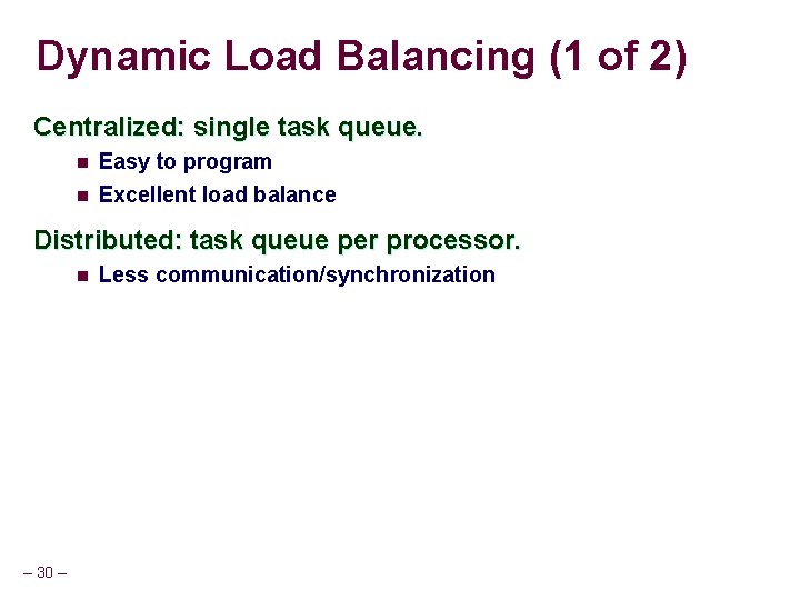
Dynamic Load Balancing (1 of 2) Centralized: single task queue. n Easy to program n Excellent load balance Distributed: task queue per processor. n – 30 – Less communication/synchronization

Dynamic Load Balancing (2 of 2) Task stealing: n n Processes normally remove and insert tasks from their own queue. When queue is empty, remove task(s) from other queues. l Extra overhead and programming difficulty. l Better load balancing. – 31 –

Semi-static Load Balancing Measure the cost of program parts. Use measurement to partition computation. Done once, done every iteration, done every n iterations. – 32 –

Summary Parallel code optimization n Critical section accesses. n Granularity. Load balance. n – 33 –