Parallel Numerical Integration Spring Semester 2005 Geoffrey Fox

Parallel Numerical Integration Spring Semester 2005 Geoffrey Fox Community Grids Laboratory Indiana University 505 N Morton Suite 224 Bloomington IN gcf@indiana. edu

Links • See Chapter 4 of Pacheco’s MPI Book • See http: //www. oldnpac. org/users/gcf/slitex/CPS 615 NI 95/index. html – For a more advanced treatment which we will highlight in these lectures • See http: //www. oldnpac. org/projects/cps 615 spring 00/presentationshtml/cps 615 nic 95/ for lectures on Romberg’s method • There is also software at http: //www. oldnpac. org/projects/cpsedu/summer 98 summary/examples/ mpi-c/mpi-c. html (Examples 1 and 2)

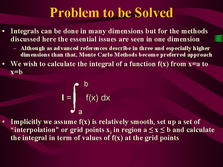
Problem to be Solved • Integrals can be done in many dimensions but for the methods discussed here the essential issues are seen in one dimension – Although as advanced references describe in three and especially higher dimensions than that, Monte Carlo Methods become preferred approach • We wish to calculate the integral of a function f(x) from x=a to x=b ∫ I= b f(x) dx a • Implicitly we assume f(x) is relatively smooth, set up a set of “interpolation” or grid points xi in region a ≤ x ≤ b and calculate the integral in term of values of f(x) at the grid points

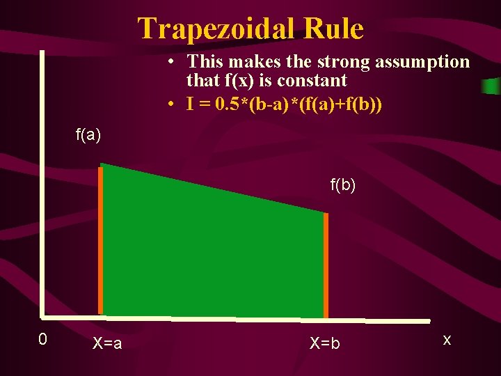
Trapezoidal Rule • This makes the strong assumption that f(x) is constant • I = 0. 5*(b-a)*(f(a)+f(b)) f(a) f(b) 0 X=a X=b x

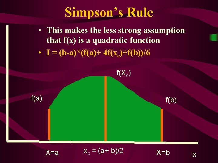
Simpson’s Rule • This makes the less strong assumption that f(x) is a quadratic function • I = (b-a)*(f(a)+ 4 f(xc)+f(b))/6 f(Xc) f(a) f(b) X=a xc = (a+ b)/2 X=b x

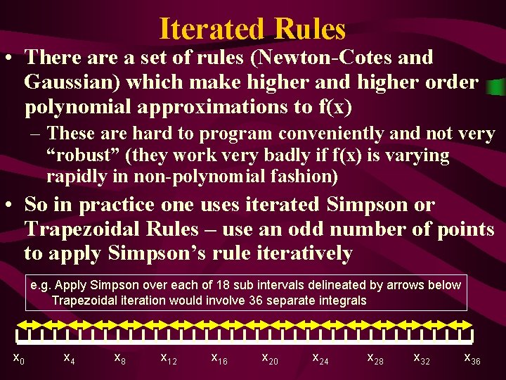
Iterated Rules • There a set of rules (Newton-Cotes and Gaussian) which make higher and higher order polynomial approximations to f(x) – These are hard to program conveniently and not very “robust” (they work very badly if f(x) is varying rapidly in non-polynomial fashion) • So in practice one uses iterated Simpson or Trapezoidal Rules – use an odd number of points to apply Simpson’s rule iteratively e. g. Apply Simpson over each of 18 sub intervals delineated by arrows below Trapezoidal iteration would involve 36 separate integrals x 0 x 4 x 8 x 12 x 16 x 20 x 24 x 28 x 32 x 36

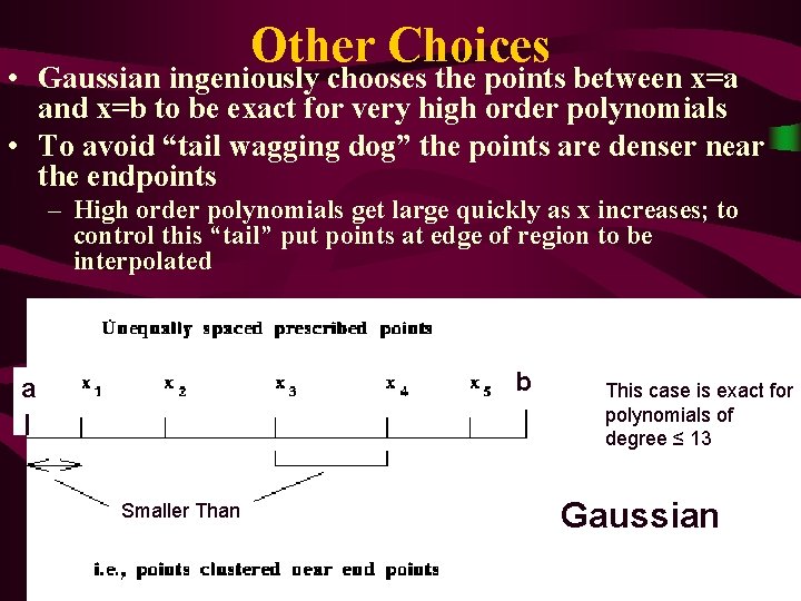
Other Choices • Gaussian ingeniously chooses the points between x=a and x=b to be exact for very high order polynomials • To avoid “tail wagging dog” the points are denser near the endpoints – High order polynomials get large quickly as x increases; to control this “tail” put points at edge of region to be interpolated b a Smaller Than This case is exact for polynomials of degree ≤ 13 Gaussian

Monte Carlo Methods • Monte Carlo (the most important) un-ingeniously chooses the points at random • The Integral is sum of the function values f(x. Random-i) at the randomly chosen x values x. Random-i multiplied by the Interval (b-a here) divided by the number of generated points • This gives the most robust method (unbiased) that is easiest to apply for multi-dimensional integrals and integrals of badly behaved functions • Funny boundaries are easy to take care of – Integrate over convenient region bigger than real region – Define function to be zero outside true integration region – Often makes function discontinuous but OK for Monte Carlo a b

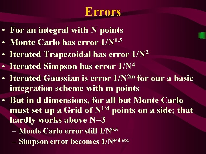
Errors • • • For an integral with N points Monte Carlo has error 1/N 0. 5 Iterated Trapezoidal has error 1/N 2 Iterated Simpson has error 1/N 4 Iterated Gaussian is error 1/N 2 m for our a basic integration scheme with m points • But in d dimensions, for all but Monte Carlo must set up a Grid of N 1/d points on a side; that hardly works above N=3 – Monte Carlo error still 1/N 0. 5 – Simpson error becomes 1/N 4/d etc.

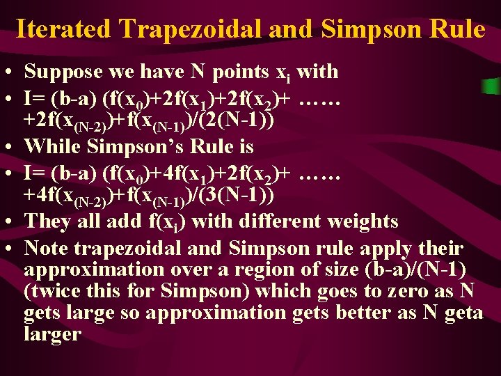
Iterated Trapezoidal and Simpson Rule • Suppose we have N points xi with • I= (b-a) (f(x 0)+2 f(x 1)+2 f(x 2)+ …… +2 f(x(N-2))+f(x(N-1))/(2(N-1)) • While Simpson’s Rule is • I= (b-a) (f(x 0)+4 f(x 1)+2 f(x 2)+ …… +4 f(x(N-2))+f(x(N-1))/(3(N-1)) • They all add f(xi) with different weights • Note trapezoidal and Simpson rule apply their approximation over a region of size (b-a)/(N-1) (twice this for Simpson) which goes to zero as N gets large so approximation gets better as N geta larger

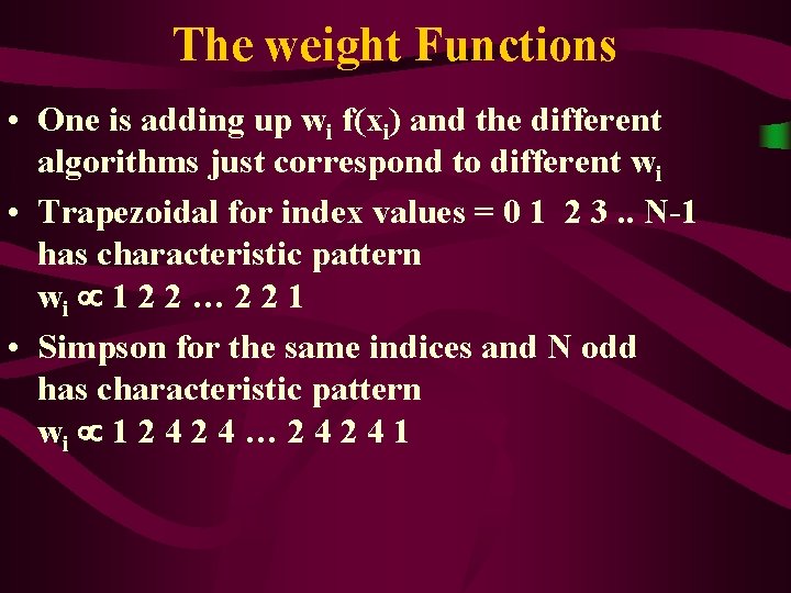
The weight Functions • One is adding up wi f(xi) and the different algorithms just correspond to different wi • Trapezoidal for index values = 0 1 2 3. . N-1 has characteristic pattern wi 1 2 2 … 2 2 1 • Simpson for the same indices and N odd has characteristic pattern wi 1 2 4 … 2 4 1

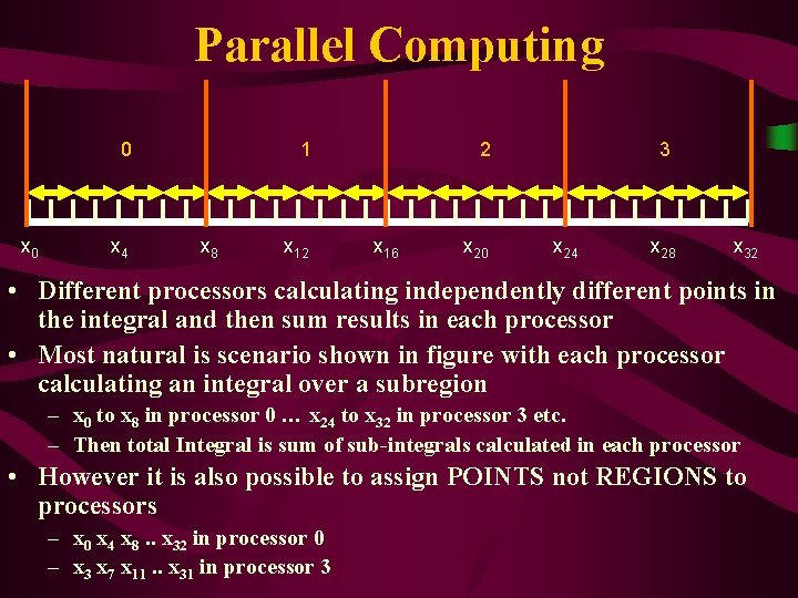
Parallel Computing 0 x 4 1 x 8 x 12 2 x 16 x 20 3 x 24 x 28 x 32 • Different processors calculating independently different points in the integral and then sum results in each processor • Most natural is scenario shown in figure with each processor calculating an integral over a subregion – x 0 to x 8 in processor 0 … x 24 to x 32 in processor 3 etc. – Then total Integral is sum of sub-integrals calculated in each processor • However it is also possible to assign POINTS not REGIONS to processors – x 0 x 4 x 8. . x 32 in processor 0 – x 3 x 7 x 11. . x 31 in processor 3

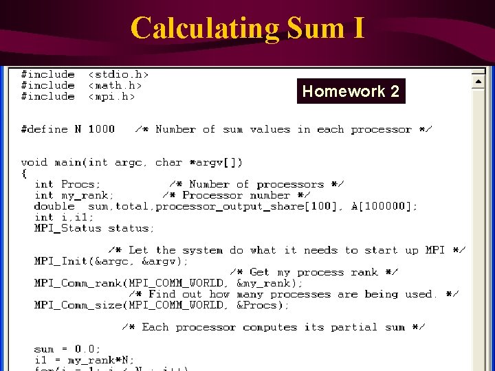
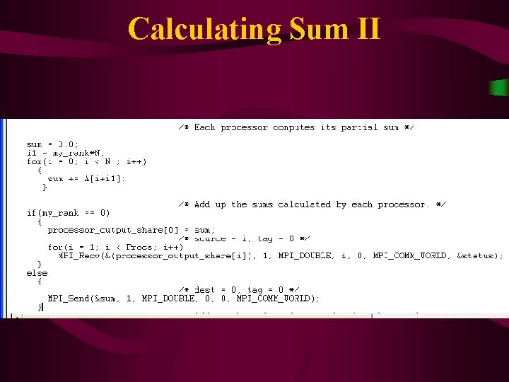
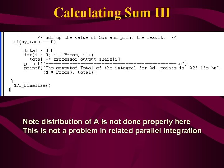
Issues in Numerical Integration for Parallel Computing • This is a classic master worker paradigm with individual processors calculating parts of the integral • They need to use MPI rank to decide which part of integration range they are responsible for • They calculate integral over this range and then we just sum their contributions over all processors – Global sum can be done by pipeline, tree or by all workers independently sending their results to the master

Calculating Sum I Homework 2

Calculating Sum II

Calculating Sum III Note distribution of A is not done properly here This is not a problem in related parallel integration

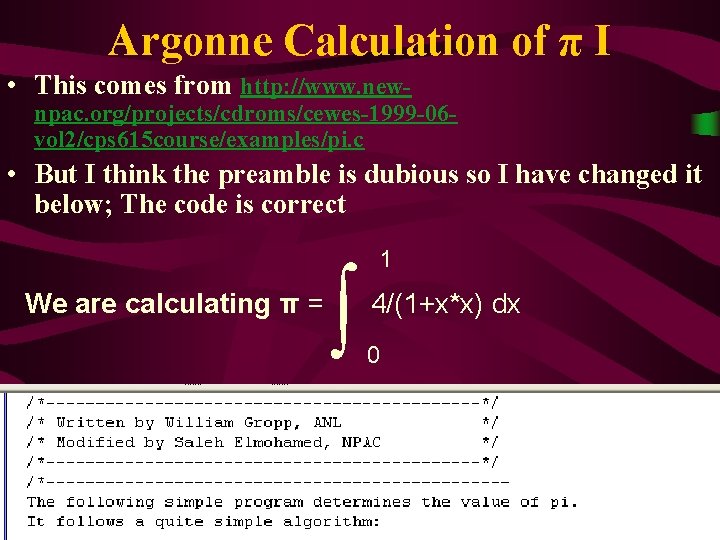
Argonne Calculation of π I • This comes from http: //www. new- npac. org/projects/cdroms/cewes-1999 -06 vol 2/cps 615 course/examples/pi. c • But I think the preamble is dubious so I have changed it below; The code is correct We are calculating π = ∫ 1 4/(1+x*x) dx 0

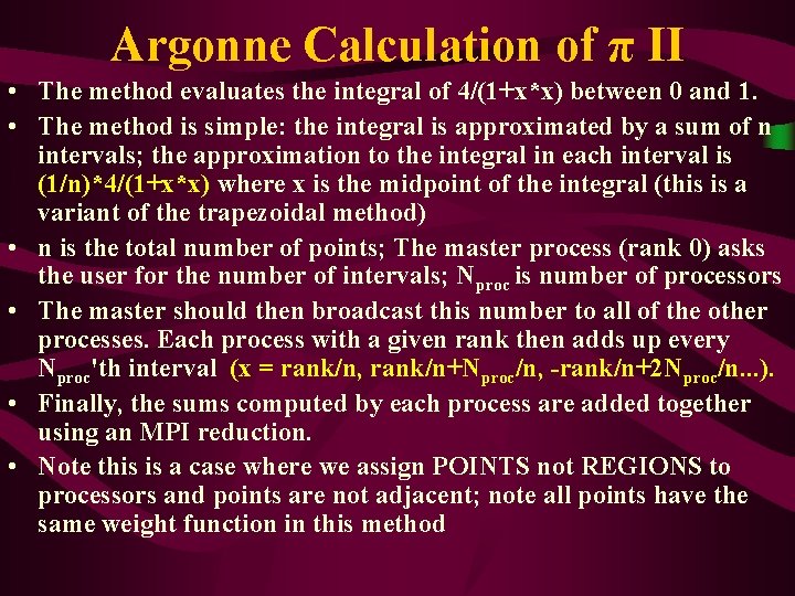
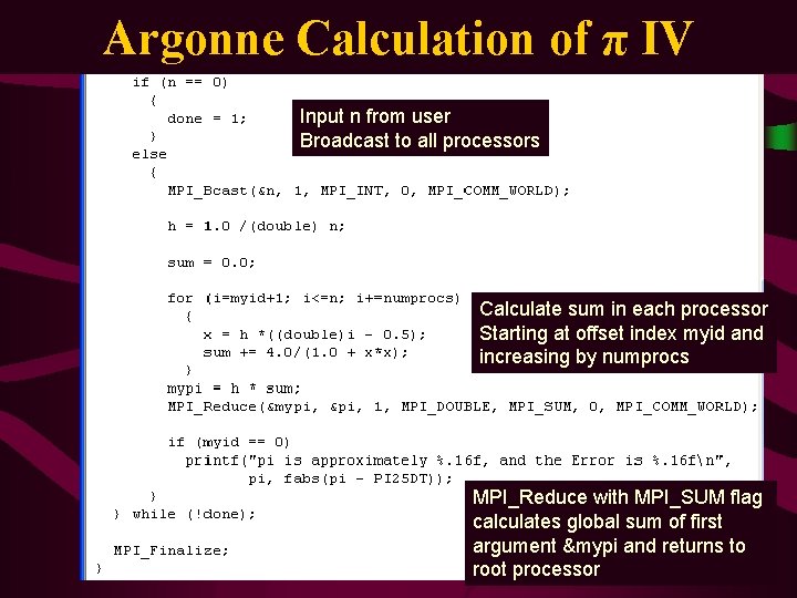
Argonne Calculation of π II • The method evaluates the integral of 4/(1+x*x) between 0 and 1. • The method is simple: the integral is approximated by a sum of n intervals; the approximation to the integral in each interval is (1/n)*4/(1+x*x) where x is the midpoint of the integral (this is a variant of the trapezoidal method) • n is the total number of points; The master process (rank 0) asks the user for the number of intervals; Nproc is number of processors • The master should then broadcast this number to all of the other processes. Each process with a given rank then adds up every Nproc'th interval (x = rank/n, rank/n+Nproc/n, -rank/n+2 Nproc/n. . . ). • Finally, the sums computed by each process are added together using an MPI reduction. • Note this is a case where we assign POINTS not REGIONS to processors and points are not adjacent; note all points have the same weight function in this method

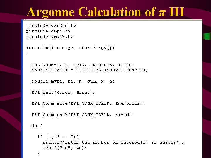
Argonne Calculation of π III

Argonne Calculation of π IV Input n from user Broadcast to all processors Calculate sum in each processor Starting at offset index myid and increasing by numprocs MPI_Reduce with MPI_SUM flag calculates global sum of first argument &mypi and returns to root processor

Simpson’s Rule I • http: //www. new-npac. org/projects/cdroms/cewes-199906 -vol 1/cps 615 course/index. html • Brief description: Using Simpson's rule we compute the value of π. When using this approach and integrating on a multiprocessor, the logical thing to do would be to partition the interval to subintervals and make each processor run on one of these subintervals. In turn, each processor applies Simpson's rule to its own interval, again, partitioning it into subintervals of equal number to the one above it, etc. Among the processors, one takes charge of receiving and adding up the results

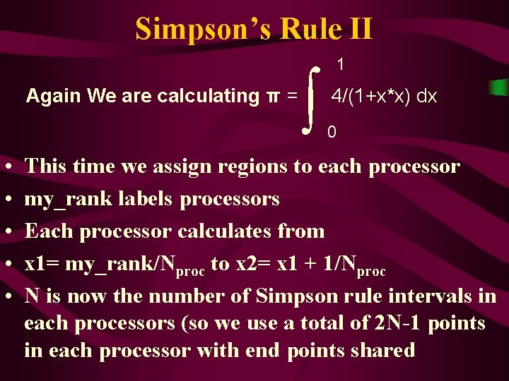
Simpson’s Rule II Again We are calculating π = • • • ∫ 1 4/(1+x*x) dx 0 This time we assign regions to each processor my_rank labels processors Each processor calculates from x 1= my_rank/Nproc to x 2= x 1 + 1/Nproc N is now the number of Simpson rule intervals in each processors (so we use a total of 2 N-1 points in each processor with end points shared

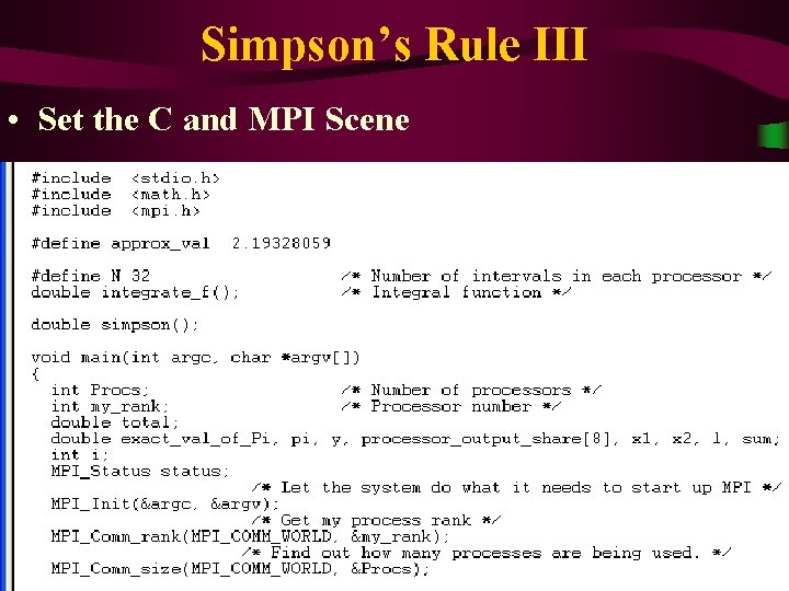
Simpson’s Rule III • Set the C and MPI Scene

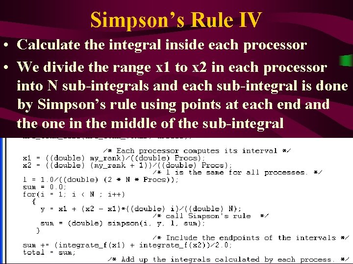
Simpson’s Rule IV • Calculate the integral inside each processor • We divide the range x 1 to x 2 in each processor into N sub-integrals and each sub-integral is done by Simpson’s rule using points at each end and the one in the middle of the sub-integral

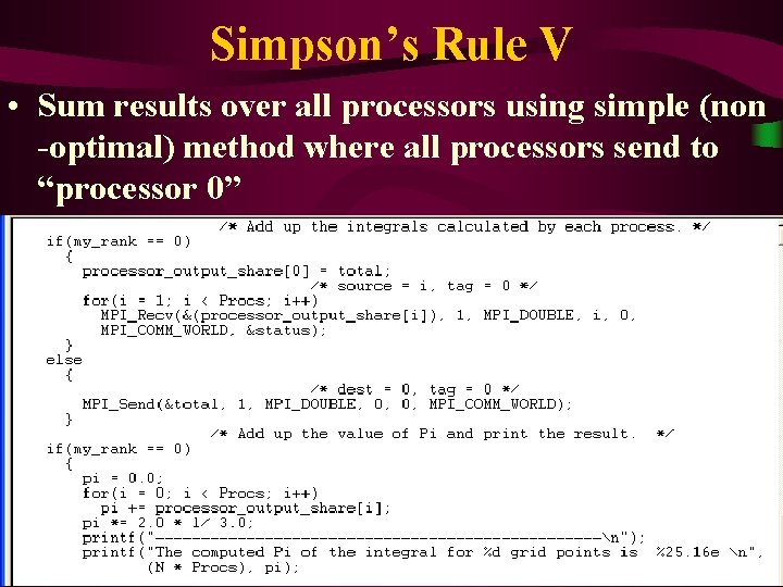
Simpson’s Rule V • Sum results over all processors using simple (non -optimal) method where all processors send to “processor 0”

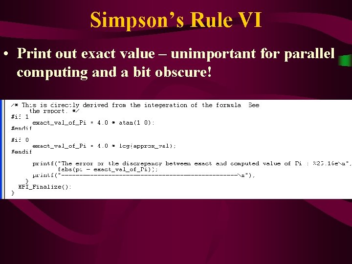
Simpson’s Rule VI • Print out exact value – unimportant for parallel computing and a bit obscure!

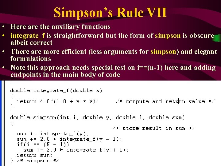
Simpson’s Rule VII • Here are the auxiliary functions • integrate_f is straightforward but the form of simpson is obscure albeit correct • There are more efficient (less arguments for simpson) and elegant formulations • Note this approach needs special test on i==(n-1) here and adding endpoints in the main body of code