Parallel Graph Algorithms Aydn Bulu ABuluclbl gov http

Parallel Graph Algorithms Aydın Buluç ABuluc@lbl. gov http: //gauss. cs. ucsb. edu/~aydin/ Lawrence Berkeley National Laboratory CS 267, Spring 2013 April 9, 2013 Slide acknowledgments: K. Madduri, J. Gilbert, D. Delling, S. Beamer

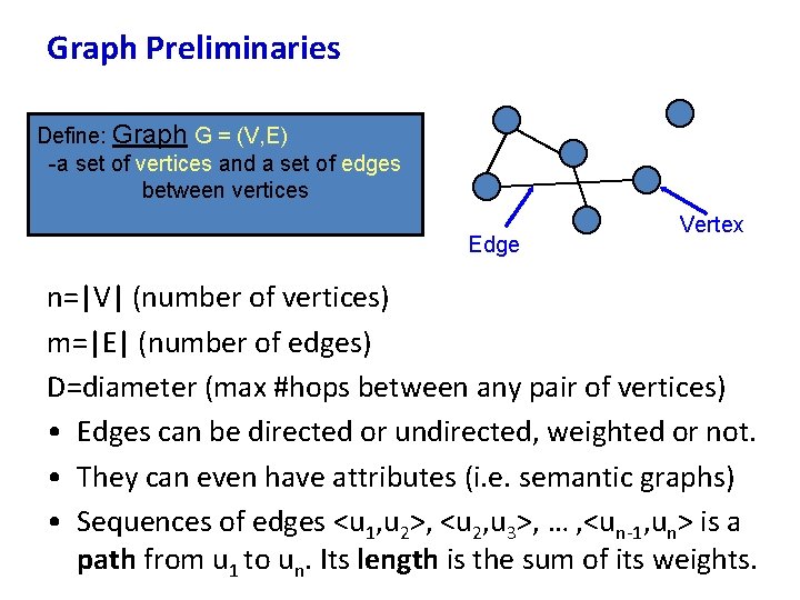
Graph Preliminaries Define: Graph G = (V, E) -a set of vertices and a set of edges between vertices Edge Vertex n=|V| (number of vertices) m=|E| (number of edges) D=diameter (max #hops between any pair of vertices) • Edges can be directed or undirected, weighted or not. • They can even have attributes (i. e. semantic graphs) • Sequences of edges <u 1, u 2>, <u 2, u 3>, … , <un-1, un> is a path from u 1 to un. Its length is the sum of its weights.

Lecture Outline • Applications • Designing parallel graph algorithms • Case studies: A. B. C. D. E. Graph traversals: Breadth-first search Shortest Paths: Delta-stepping, PHAST, Floyd-Warshall Ranking: Betweenness centrality Maximal Independent Sets: Luby’s algorithm Strongly Connected Components • Wrap-up: challenges on current systems

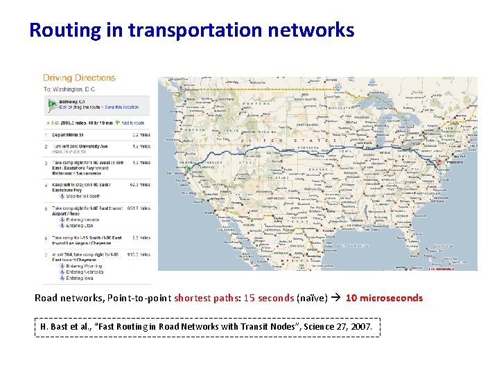
Routing in transportation networks Road networks, Point-to-point shortest paths: 15 seconds (naïve) 10 microseconds H. Bast et al. , “Fast Routing in Road Networks with Transit Nodes”, Science 27, 2007.

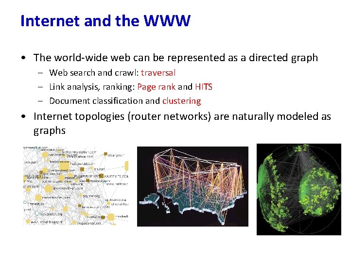
Internet and the WWW • The world-wide web can be represented as a directed graph – Web search and crawl: traversal – Link analysis, ranking: Page rank and HITS – Document classification and clustering • Internet topologies (router networks) are naturally modeled as graphs

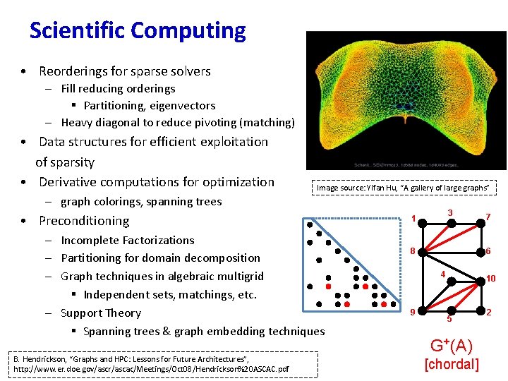
Scientific Computing • Reorderings for sparse solvers – Fill reducing orderings § Partitioning, eigenvectors – Heavy diagonal to reduce pivoting (matching) • Data structures for efficient exploitation of sparsity • Derivative computations for optimization Image source: Yifan Hu, “A gallery of large graphs” – graph colorings, spanning trees • Preconditioning – Incomplete Factorizations – Partitioning for domain decomposition – Graph techniques in algebraic multigrid § Independent sets, matchings, etc. – Support Theory § Spanning trees & graph embedding techniques B. Hendrickson, “Graphs and HPC: Lessons for Future Architectures”, http: //www. er. doe. gov/ascr/ascac/Meetings/Oct 08/Hendrickson%20 ASCAC. pdf 3 1 6 8 4 9 7 10 5 G+(A) [chordal] 2

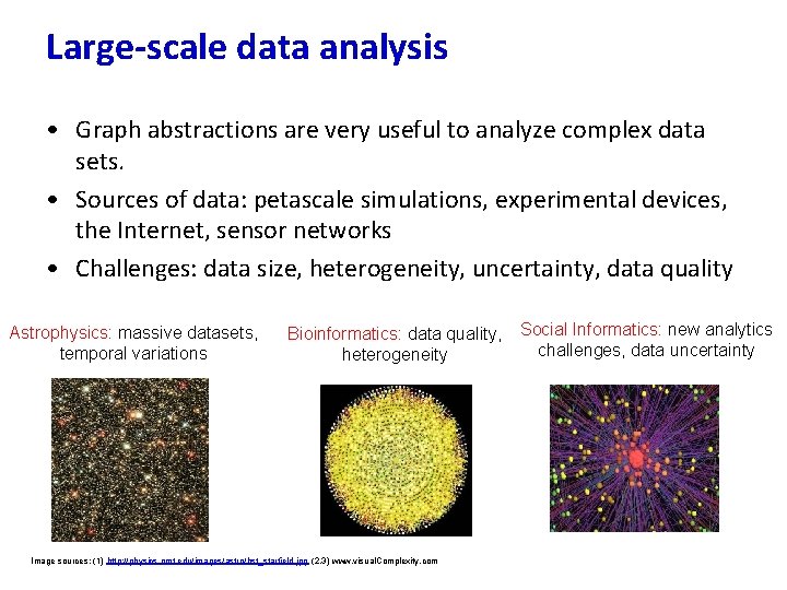
Large-scale data analysis • Graph abstractions are very useful to analyze complex data sets. • Sources of data: petascale simulations, experimental devices, the Internet, sensor networks • Challenges: data size, heterogeneity, uncertainty, data quality Astrophysics: massive datasets, temporal variations Bioinformatics: data quality, heterogeneity Image sources: (1) http: //physics. nmt. edu/images/astro/hst_starfield. jpg (2, 3) www. visual. Complexity. com Social Informatics: new analytics challenges, data uncertainty

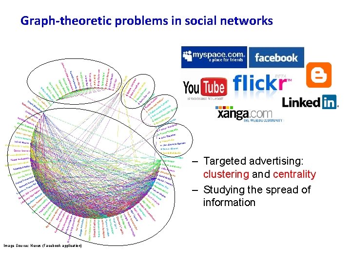
Graph-theoretic problems in social networks – Targeted advertising: clustering and centrality – Studying the spread of information Image Source: Nexus (Facebook application)

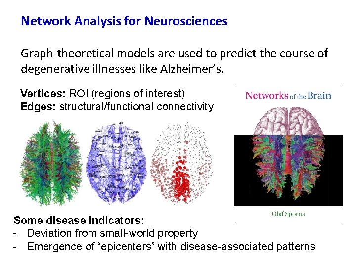
Network Analysis for Neurosciences Graph-theoretical models are used to predict the course of degenerative illnesses like Alzheimer’s. Vertices: ROI (regions of interest) Edges: structural/functional connectivity Some disease indicators: - Deviation from small-world property - Emergence of “epicenters” with disease-associated patterns

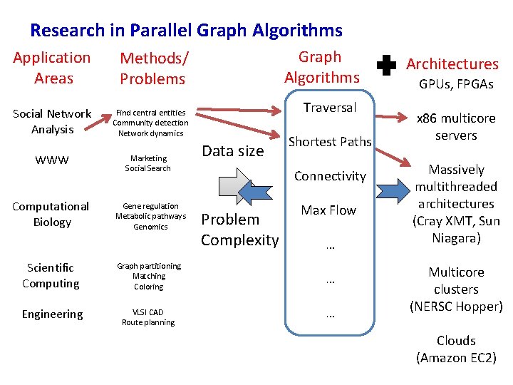
Research in Parallel Graph Algorithms Application Areas Social Network Analysis Graph Algorithms Methods/ Problems Traversal Find central entities Community detection Network dynamics WWW Marketing Social Search Computational Biology Gene regulation Metabolic pathways Genomics Scientific Computing Graph partitioning Matching Coloring Engineering VLSI CAD Route planning Data size Shortest Paths Connectivity Problem Complexity Max Flow … … … Architectures GPUs, FPGAs x 86 multicore servers Massively multithreaded architectures (Cray XMT, Sun Niagara) Multicore clusters (NERSC Hopper) Clouds (Amazon EC 2)

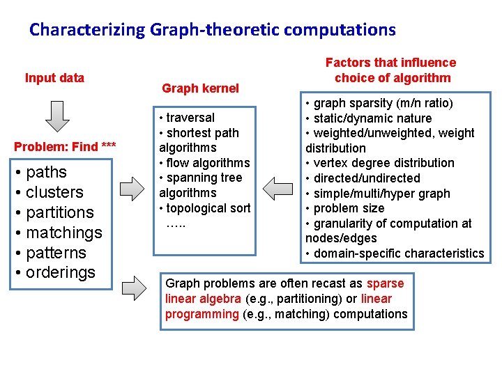
Characterizing Graph-theoretic computations Input data Problem: Find *** • paths • clusters • partitions • matchings • patterns • orderings Graph kernel • traversal • shortest path algorithms • flow algorithms • spanning tree algorithms • topological sort …. . Factors that influence choice of algorithm • graph sparsity (m/n ratio) • static/dynamic nature • weighted/unweighted, weight distribution • vertex degree distribution • directed/undirected • simple/multi/hyper graph • problem size • granularity of computation at nodes/edges • domain-specific characteristics Graph problems are often recast as sparse linear algebra (e. g. , partitioning) or linear programming (e. g. , matching) computations

Lecture Outline • Applications • Designing parallel graph algorithms • Case studies: A. B. C. D. E. Graph traversals: Breadth-first search Shortest Paths: Delta-stepping, PHAST, Floyd-Warshall Ranking: Betweenness centrality Maximal Independent Sets: Luby’s algorithm Strongly Connected Components • Wrap-up: challenges on current systems

The PRAM model • Many PRAM graph algorithms in 1980 s. • Idealized parallel shared memory system model • Unbounded number of synchronous processors; no synchronization, communication cost; no parallel overhead • EREW (Exclusive Read Exclusive Write), CREW (Concurrent Read Exclusive Write) • Measuring performance: space and time complexity; total number of operations (work)

PRAM Pros and Cons • Pros – Simple and clean semantics. – The majority of theoretical parallel algorithms are designed using the PRAM model. – Independent of the communication network topology. • Cons – – – Not realistic, too powerful communication model. Communication costs are ignored. Synchronized processors. No local memory. Big-O notation is often misleading.

Building blocks of classical PRAM graph algorithms • Prefix sums • Symmetry breaking • Pointer jumping • List ranking • Euler tours • Vertex collapse • Tree contraction [some covered in the “Tricks with Trees” lecture]

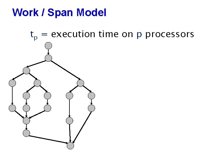
Work / Span Model tp = execution time on p processors

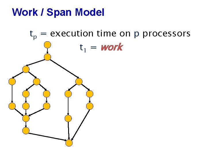
Work / Span Model tp = execution time on p processors t 1 = work

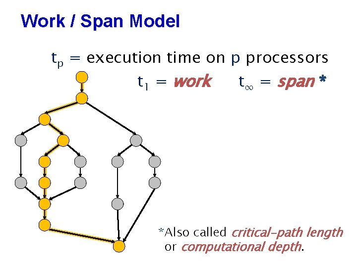
Work / Span Model tp = execution time on p processors t 1 = work t∞ = span * *Also called critical-path length or computational depth.

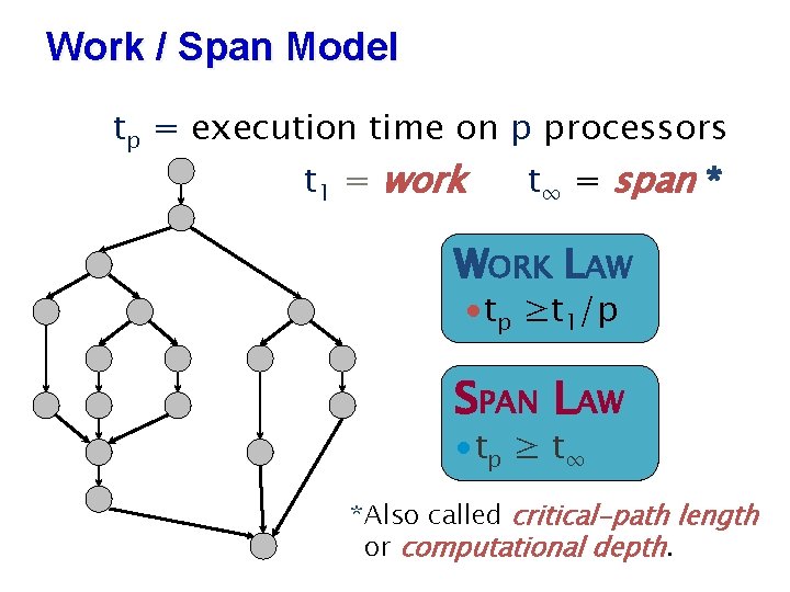
Work / Span Model tp = execution time on p processors t 1 = work t∞ = span * WORK LAW ∙tp ≥t 1/p SPAN LAW ∙ tp ≥ t ∞ *Also called critical-path length or computational depth.

Data structures: graph representation Static case • Dense graphs (m = Θ(n 2)): adjacency matrix commonly used. • Sparse graphs: adjacency lists, compressed sparse matrices Dynamic • representation depends on common-case query • Edge insertions or deletions? Vertex insertions or deletions? Edge weight updates? • Graph update rate • Queries: connectivity, paths, flow, etc. • Optimizing for locality a key design consideration.

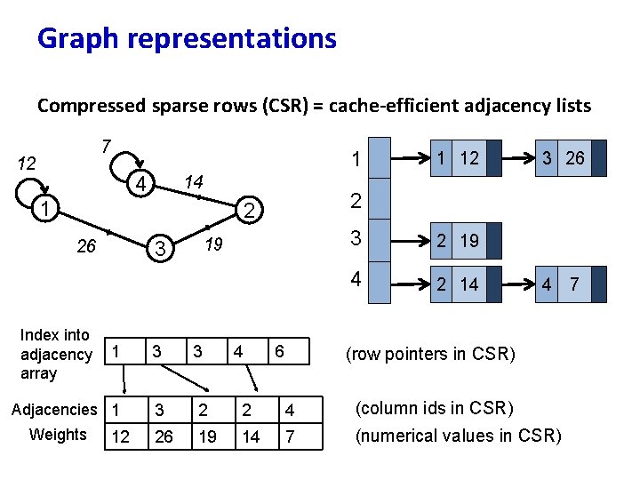
Graph representations Compressed sparse rows (CSR) = cache-efficient adjacency lists 7 12 1 4 14 1 Index into adjacency array 19 3 6 2 19 4 2 14 4 3 Adjacencies 1 3 2 2 4 (column ids in CSR) 26 19 14 7 (numerical values in CSR) 12 4 3 1 Weights 3 3 26 2 2 26 1 12 (row pointers in CSR) 7

Distributed graph representations • Each processor stores the entire graph (“full replication”) • Each processor stores n/p vertices and all adjacencies out of these vertices (“ 1 D partitioning”) • How to create these “p” vertex partitions? – Graph partitioning algorithms: recursively optimize for conductance (edge cut/size of smaller partition) – Randomly shuffling the vertex identifiers ensures that edge count/processor are roughly the same

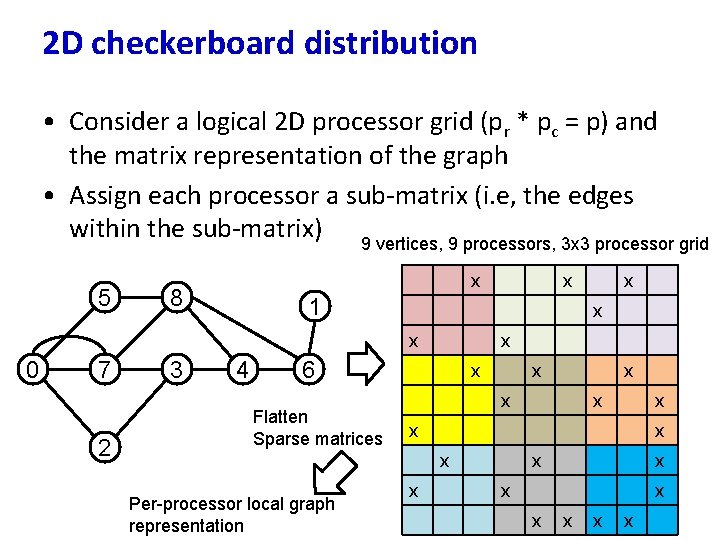
2 D checkerboard distribution • Consider a logical 2 D processor grid (pr * pc = p) and the matrix representation of the graph • Assign each processor a sub-matrix (i. e, the edges within the sub-matrix) 9 vertices, 9 processors, 3 x 3 processor grid 5 x 8 1 7 2 3 4 x 6 Flatten Sparse matrices x x x x x Per-processor local graph representation x x x 0 x x x x x

High-performance graph algorithms • Implementations are typically array-based for performance (e. g. CSR representation). • Concurrency = minimize synchronization (span) • Where is the data? Find the distribution that minimizes inter-processor communication. • Memory access patterns – Regularize them (spatial locality) – Minimize DRAM traffic (temporal locality) • Work-efficiency – Is (Parallel time) * (# of processors) = (Serial work)?

Lecture Outline • Applications • Designing parallel graph algorithms • Case studies: A. B. C. D. E. Graph traversals: Breadth-first search Shortest Paths: Delta-stepping, PHAST, Floyd-Warshall Ranking: Betweenness centrality Maximal Independent Sets: Luby’s algorithm Strongly Connected Components • Wrap-up: challenges on current systems

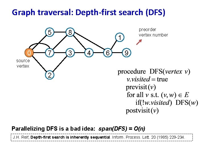
Graph traversal: Depth-first search (DFS) 9 5 8 8 0 source vertex 7 7 1 2 3 3 4 4 6 preorder vertex number 6 5 9 1 2 Parallelizing DFS is a bad idea: span(DFS) = O(n) J. H. Reif, Depth-first search is inherently sequential. Inform. Process. Lett. 20 (1985) 229 -234.

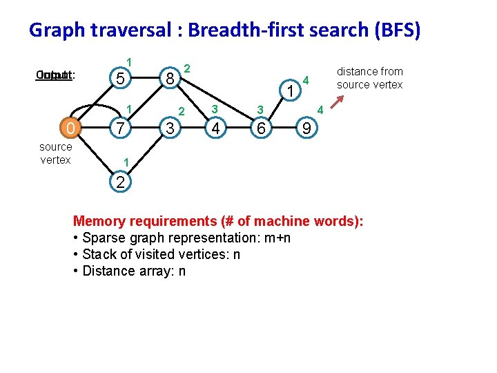
Graph traversal : Breadth-first search (BFS) 1 Input: Output: 5 8 1 0 source vertex 7 2 1 2 3 3 3 4 6 distance from source vertex 4 4 9 1 2 Memory requirements (# of machine words): • Sparse graph representation: m+n • Stack of visited vertices: n • Distance array: n

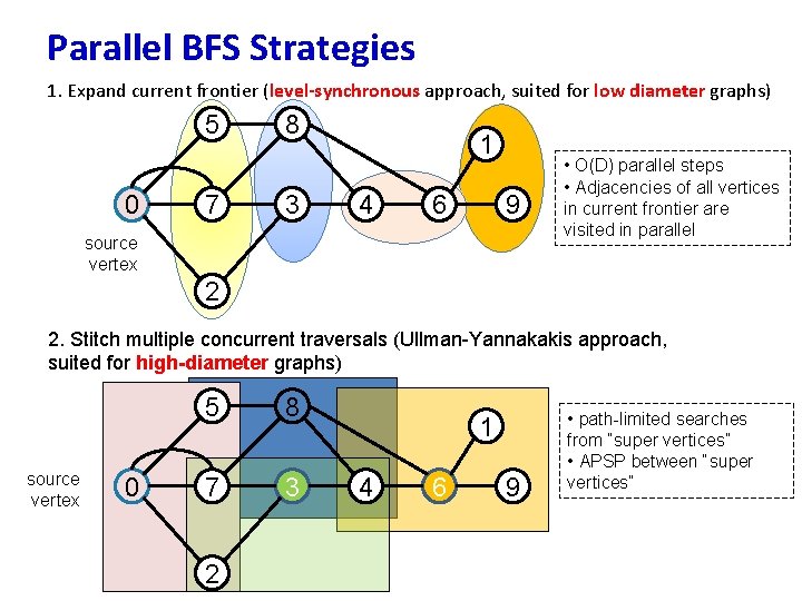
Parallel BFS Strategies 1. Expand current frontier (level-synchronous approach, suited for low diameter graphs) 5 0 7 8 3 1 4 6 9 source vertex • O(D) parallel steps • Adjacencies of all vertices in current frontier are visited in parallel 2 2. Stitch multiple concurrent traversals (Ullman-Yannakakis approach, suited for high-diameter graphs) source vertex 0 5 8 7 3 2 1 4 6 9 • path-limited searches from “super vertices” • APSP between “super vertices”

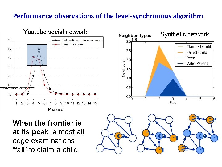
Performance observations of the level-synchronous algorithm Youtube social network When the frontier is at its peak, almost all edge examinations “fail” to claim a child Synthetic network

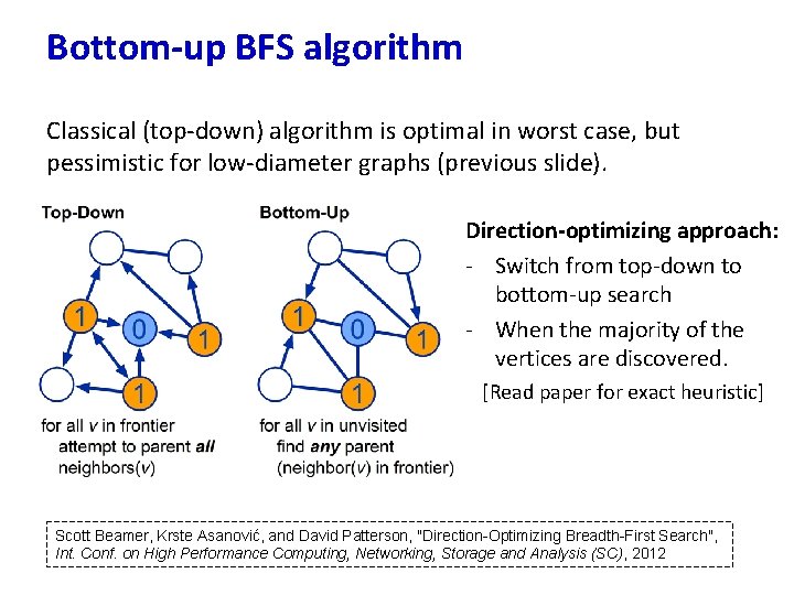
Bottom-up BFS algorithm Classical (top-down) algorithm is optimal in worst case, but pessimistic for low-diameter graphs (previous slide). Direction-optimizing approach: - Switch from top-down to bottom-up search - When the majority of the vertices are discovered. [Read paper for exact heuristic] Scott Beamer, Krste Asanović, and David Patterson, "Direction-Optimizing Breadth-First Search", Int. Conf. on High Performance Computing, Networking, Storage and Analysis (SC), 2012

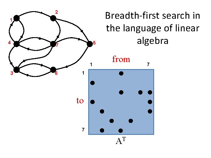
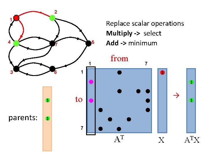
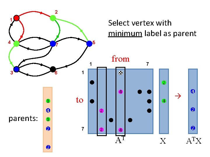
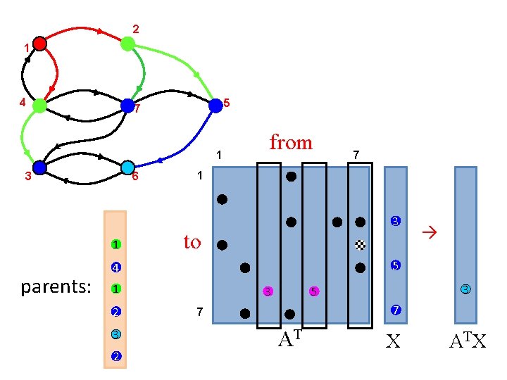
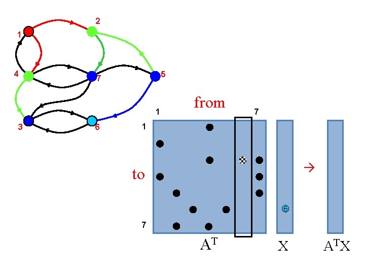
2 1 4 5 7 1 3 6 Breadth-first search in the language of linear algebra from 1 to 7 AT 7

2 1 4 5 7 1 6 3 Replace scalar operations Multiply -> select Add -> minimum from 7 1 1 parents: to 1 1 7 AT X

2 1 Select vertex with minimum label as parent 4 5 7 from 1 6 3 7 1 2 1 parents: 4 to 4 4 4 2 2 1 2 2 7 2 2 4 AT X

2 1 4 5 7 1 6 3 1 parents: from 1 3 to 1 3 2 5 4 2 7 3 5 3 7 7 AT X

2 1 4 5 7 1 3 6 from 7 1 to 6 7 AT X

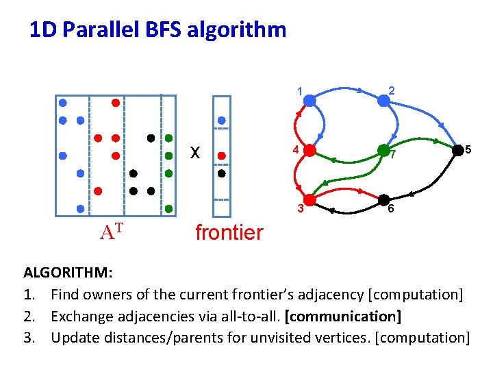
1 D Parallel BFS algorithm 1 x 4 3 AT 2 7 5 6 xfrontier ALGORITHM: 1. Find owners of the current frontier’s adjacency [computation] 2. Exchange adjacencies via all-to-all. [communication] 3. Update distances/parents for unvisited vertices. [computation]

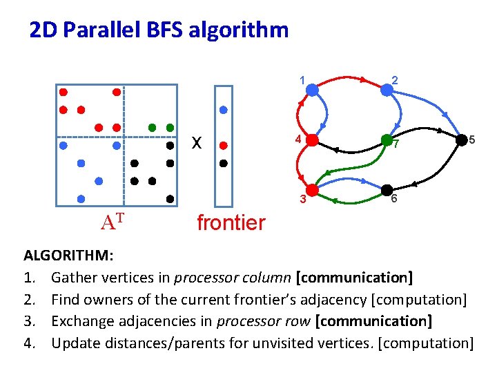
2 D Parallel BFS algorithm 1 x 4 3 AT 2 7 5 6 xfrontier ALGORITHM: 1. Gather vertices in processor column [communication] 2. Find owners of the current frontier’s adjacency [computation] 3. Exchange adjacencies in processor row [communication] 4. Update distances/parents for unvisited vertices. [computation]

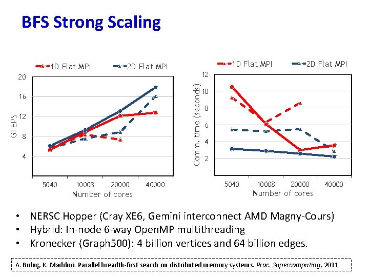
BFS Strong Scaling 1 D Flat MPI 2 D Flat MPI 12 Comm. time (seconds) 20 GTEPS 16 12 8 4 5040 10008 20000 Number of cores 40000 2 D Flat MPI 10 8 6 4 2 5040 10008 20000 40000 Number of cores • NERSC Hopper (Cray XE 6, Gemini interconnect AMD Magny-Cours) • Hybrid: In-node 6 -way Open. MP multithreading • Kronecker (Graph 500): 4 billion vertices and 64 billion edges. A. Buluç, K. Madduri. Parallel breadth-first search on distributed memory systems. Proc. Supercomputing, 2011.

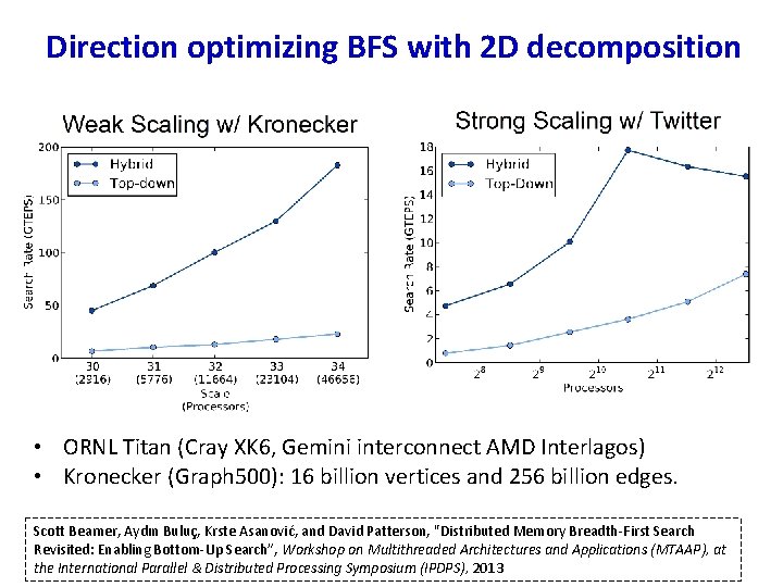
Direction optimizing BFS with 2 D decomposition • ORNL Titan (Cray XK 6, Gemini interconnect AMD Interlagos) • Kronecker (Graph 500): 16 billion vertices and 256 billion edges. Scott Beamer, Aydın Buluç, Krste Asanović, and David Patterson, "Distributed Memory Breadth-First Search Revisited: Enabling Bottom-Up Search”, Workshop on Multithreaded Architectures and Applications (MTAAP), at the International Parallel & Distributed Processing Symposium (IPDPS), 2013

Lecture Outline • Applications • Designing parallel graph algorithms • Case studies: A. B. C. D. E. Graph traversals: Breadth-first search Shortest Paths: Delta-stepping, PHAST, Floyd-Warshall Ranking: Betweenness centrality Maximal Independent Sets: Luby’s algorithm Strongly Connected Components • Wrap-up: challenges on current systems

Parallel Single-source Shortest Paths (SSSP) algorithms • Famous serial algorithms: – Bellman-Ford : label correcting - works on any graph – Dijkstra : label setting – requires nonnegative edge weights • No known PRAM algorithm that runs in sub-linear time and O(m+n log n) work • Ullman-Yannakakis randomized approach • Meyer and Sanders, ∆ - stepping algorithm • Distributed memory implementations based on graph partitioning • Heuristics for load balancing and termination detection K. Madduri, D. A. Bader, J. W. Berry, and J. R. Crobak, “An Experimental Study of A Parallel Shortest Path Algorithm for Solving Large-Scale Graph Instances, ” Workshop on Algorithm Engineering and Experiments (ALENEX), New Orleans, LA, January 6, 2007.

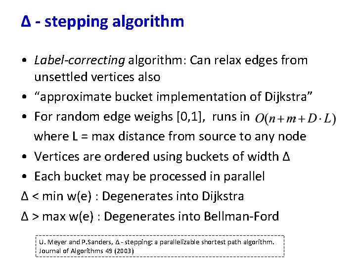
∆ - stepping algorithm • Label-correcting algorithm: Can relax edges from unsettled vertices also • “approximate bucket implementation of Dijkstra” • For random edge weighs [0, 1], runs in where L = max distance from source to any node • Vertices are ordered using buckets of width ∆ • Each bucket may be processed in parallel ∆ < min w(e) : Degenerates into Dijkstra ∆ > max w(e) : Degenerates into Bellman-Ford U. Meyer and P. Sanders, ∆ - stepping: a parallelizable shortest path algorithm. Journal of Algorithms 49 (2003)

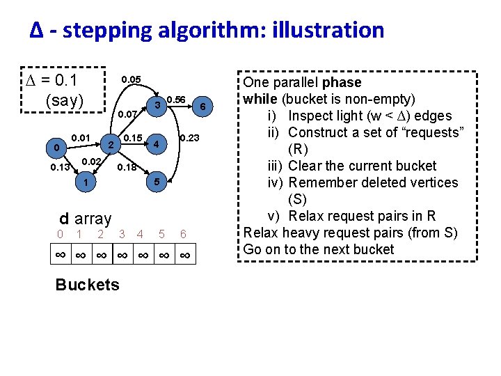
∆ - stepping algorithm: illustration ∆ = 0. 1 (say) 0 0. 05 0. 07 0. 01 0. 02 0. 13 0. 15 2 3 0. 56 0. 23 4 0. 18 5 1 d array 0 1 2 3 4 5 6 ∞ ∞ ∞ ∞ Buckets 6 One parallel phase while (bucket is non-empty) i) Inspect light (w < ∆) edges ii) Construct a set of “requests” (R) iii) Clear the current bucket iv) Remember deleted vertices (S) v) Relax request pairs in R Relax heavy request pairs (from S) Go on to the next bucket

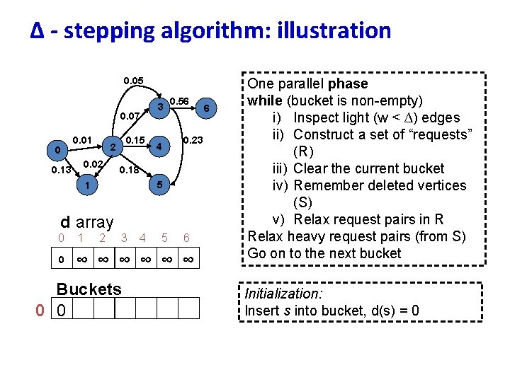
∆ - stepping algorithm: illustration 0. 05 0. 07 0 0. 01 0. 02 0. 13 0. 15 2 3 0. 56 0. 23 4 0. 18 5 1 d array 0 1 2 3 0 ∞ ∞ ∞ Buckets 0 0 4 5 6 6 One parallel phase while (bucket is non-empty) i) Inspect light (w < ∆) edges ii) Construct a set of “requests” (R) iii) Clear the current bucket iv) Remember deleted vertices (S) v) Relax request pairs in R Relax heavy request pairs (from S) Go on to the next bucket Initialization: Insert s into bucket, d(s) = 0

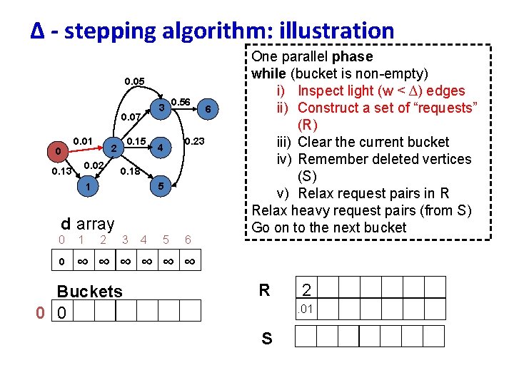
∆ - stepping algorithm: illustration 0. 05 0. 07 0 0. 01 0. 02 0. 13 0. 15 2 3 0. 56 0. 23 4 0. 18 5 1 d array 0 1 2 3 0 ∞ ∞ ∞ Buckets 0 0 4 5 6 6 One parallel phase while (bucket is non-empty) i) Inspect light (w < ∆) edges ii) Construct a set of “requests” (R) iii) Clear the current bucket iv) Remember deleted vertices (S) v) Relax request pairs in R Relax heavy request pairs (from S) Go on to the next bucket R 2. 01 S

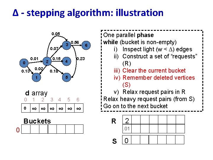
∆ - stepping algorithm: illustration 0. 05 0. 07 0 0. 01 0. 02 0. 13 0. 15 2 3 0. 56 0. 23 4 0. 18 5 1 d array 0 1 2 3 0 ∞ ∞ ∞ Buckets 4 5 6 6 One parallel phase while (bucket is non-empty) i) Inspect light (w < ∆) edges ii) Construct a set of “requests” (R) iii) Clear the current bucket iv) Remember deleted vertices (S) v) Relax request pairs in R Relax heavy request pairs (from S) Go on to the next bucket R 0 2. 01 S 0

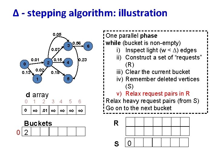
∆ - stepping algorithm: illustration 0. 05 0. 07 0 0. 01 0. 02 0. 13 0. 15 2 3 0. 56 0. 23 4 0. 18 5 1 d array 0 1 2 3 0 ∞ . 01 ∞ ∞ Buckets 0 2 4 5 6 6 One parallel phase while (bucket is non-empty) i) Inspect light (w < ∆) edges ii) Construct a set of “requests” (R) iii) Clear the current bucket iv) Remember deleted vertices (S) v) Relax request pairs in R Relax heavy request pairs (from S) Go on to the next bucket R S 0

∆ - stepping algorithm: illustration 0. 05 0. 07 0 0. 01 0. 02 0. 13 0. 15 2 3 0. 56 0. 23 4 0. 18 5 1 d array 0 1 2 3 0 ∞ . 01 ∞ ∞ Buckets 0 2 4 5 6 6 One parallel phase while (bucket is non-empty) i) Inspect light (w < ∆) edges ii) Construct a set of “requests” (R) iii) Clear the current bucket iv) Remember deleted vertices (S) v) Relax request pairs in R Relax heavy request pairs (from S) Go on to the next bucket R 1 3. 06 S 0

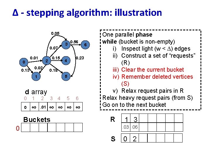
∆ - stepping algorithm: illustration 0. 05 0. 07 0 0. 01 0. 02 0. 13 0. 15 2 3 0. 56 0. 23 4 0. 18 5 1 d array 0 1 2 3 0 ∞ . 01 ∞ ∞ Buckets 4 5 6 6 One parallel phase while (bucket is non-empty) i) Inspect light (w < ∆) edges ii) Construct a set of “requests” (R) iii) Clear the current bucket iv) Remember deleted vertices (S) v) Relax request pairs in R Relax heavy request pairs (from S) Go on to the next bucket R 0 1 3. 06 S 0 2

∆ - stepping algorithm: illustration 0. 05 3 0. 07 0 0. 01 0. 02 0. 13 0. 15 2 0. 56 0. 23 4 0. 18 5 1 d array 0 1 2 3 0 . 03. 01. 06 Buckets 0 1 3 4 5 6 ∞ ∞ ∞ 6 One parallel phase while (bucket is non-empty) i) Inspect light (w < ∆) edges ii) Construct a set of “requests” (R) iii) Clear the current bucket iv) Remember deleted vertices (S) v) Relax request pairs in R Relax heavy request pairs (from S) Go on to the next bucket R S 0 2

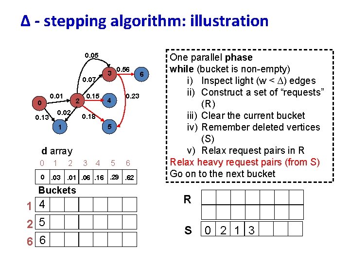
∆ - stepping algorithm: illustration 0. 05 0. 07 0 0. 01 2 0. 02 0. 13 0. 15 3 0. 56 0. 23 4 0. 18 5 1 d array 0 1 2 3 4 5 6 0. 03. 01. 06. 16. 29. 62 Buckets 1 4 2 5 6 6 6 One parallel phase while (bucket is non-empty) i) Inspect light (w < ∆) edges ii) Construct a set of “requests” (R) iii) Clear the current bucket iv) Remember deleted vertices (S) v) Relax request pairs in R Relax heavy request pairs (from S) Go on to the next bucket R S 0 2 1 3

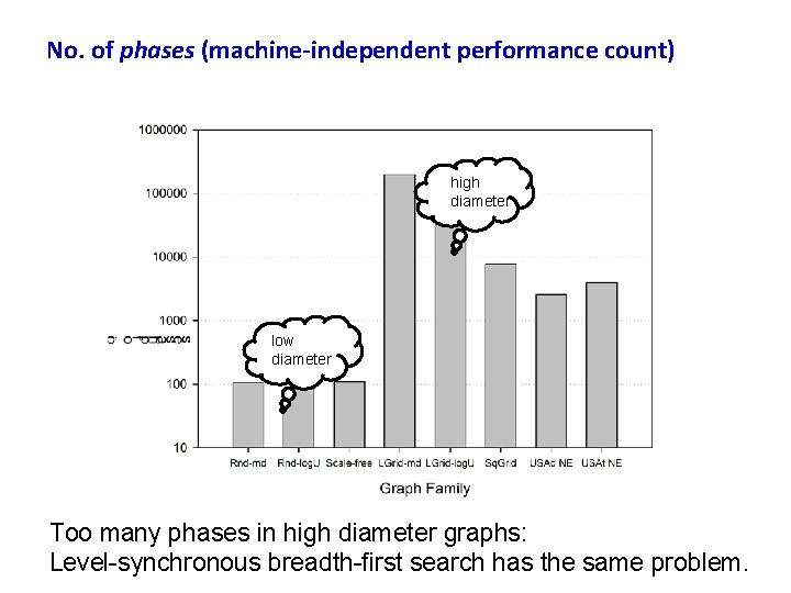
No. of phases (machine-independent performance count) high diameter low diameter Too many phases in high diameter graphs: Level-synchronous breadth-first search has the same problem.

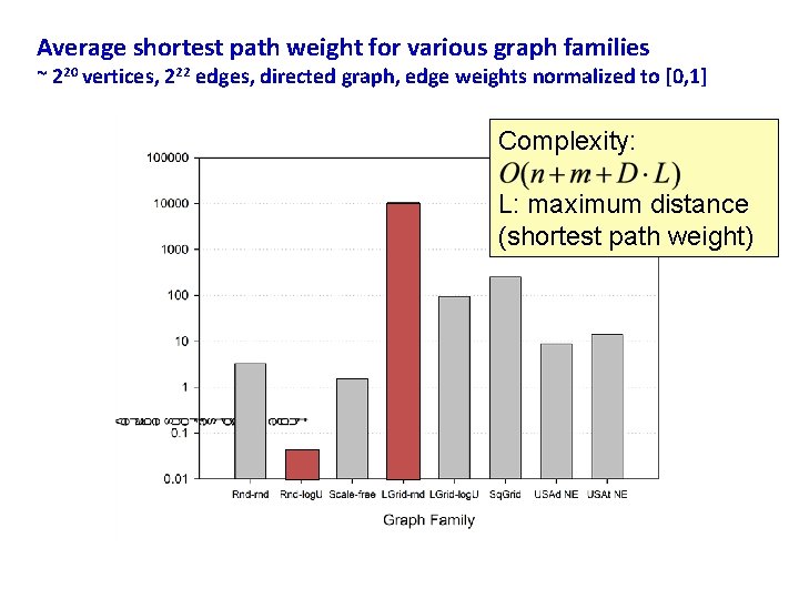
Average shortest path weight for various graph families ~ 220 vertices, 222 edges, directed graph, edge weights normalized to [0, 1] Complexity: L: maximum distance (shortest path weight)

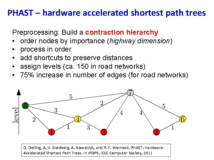
PHAST – hardware accelerated shortest path trees Preprocessing: Build a contraction hierarchy • order nodes by importance (highway dimension) • process in order • add shortcuts to preserve distances • assign levels (ca. 150 in road networks) • 75% increase in number of edges (for road networks) D. Delling, A. V. Goldberg, A. Nowatzyk, and R. F. Werneck. PHAST: Hardware- Accelerated Shortest Path Trees. In IPDPS. IEEE Computer Society, 2011

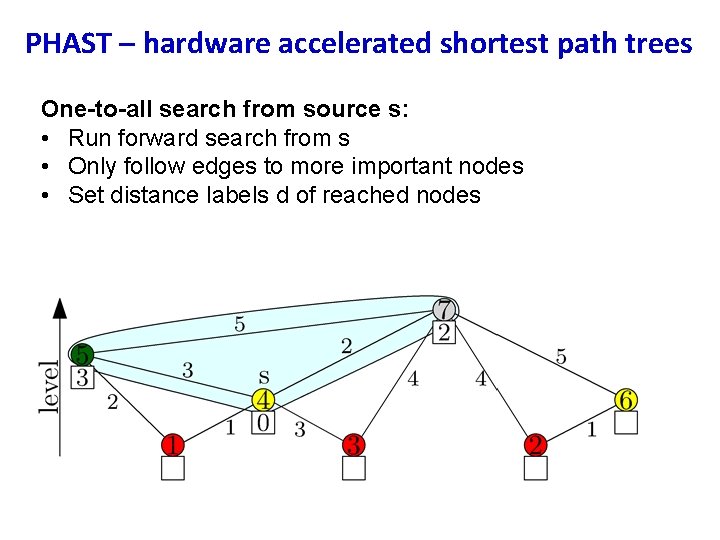
PHAST – hardware accelerated shortest path trees One-to-all search from source s: • Run forward search from s • Only follow edges to more important nodes • Set distance labels d of reached nodes

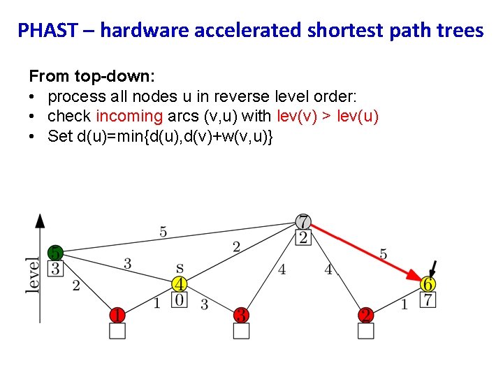
PHAST – hardware accelerated shortest path trees From top-down: • process all nodes u in reverse level order: • check incoming arcs (v, u) with lev(v) > lev(u) • Set d(u)=min{d(u), d(v)+w(v, u)}

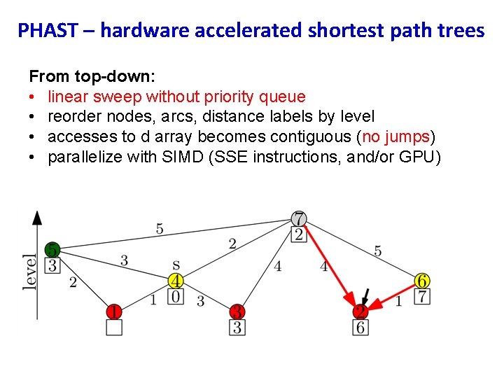
PHAST – hardware accelerated shortest path trees From top-down: • linear sweep without priority queue • reorder nodes, arcs, distance labels by level • accesses to d array becomes contiguous (no jumps) • parallelize with SIMD (SSE instructions, and/or GPU)

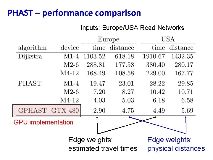
PHAST – performance comparison Inputs: Europe/USA Road Networks GPU implementation Edge weights: estimated travel times Edge weights: physical distances

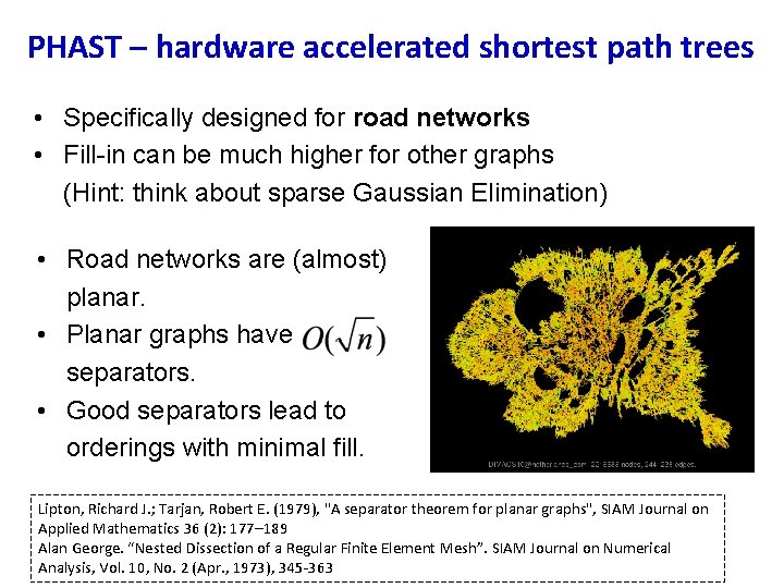
PHAST – hardware accelerated shortest path trees • Specifically designed for road networks • Fill-in can be much higher for other graphs (Hint: think about sparse Gaussian Elimination) • Road networks are (almost) planar. • Planar graphs have separators. • Good separators lead to orderings with minimal fill. Lipton, Richard J. ; Tarjan, Robert E. (1979), "A separator theorem for planar graphs", SIAM Journal on Applied Mathematics 36 (2): 177– 189 Alan George. “Nested Dissection of a Regular Finite Element Mesh”. SIAM Journal on Numerical Analysis, Vol. 10, No. 2 (Apr. , 1973), 345 -363

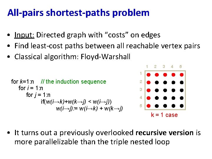
All-pairs shortest-paths problem • Input: Directed graph with “costs” on edges • Find least-cost paths between all reachable vertex pairs • Classical algorithm: Floyd-Warshall 1 2 3 4 5 1 for k=1: n // the induction sequence for i = 1: n for j = 1: n if(w(i→k)+w(k→j) < w(i→j)) w(i→j): = w(i→k) + w(k→j) 2 3 4 5 k = 1 case • It turns out a previously overlooked recursive version is more parallelizable than the triple nested loop

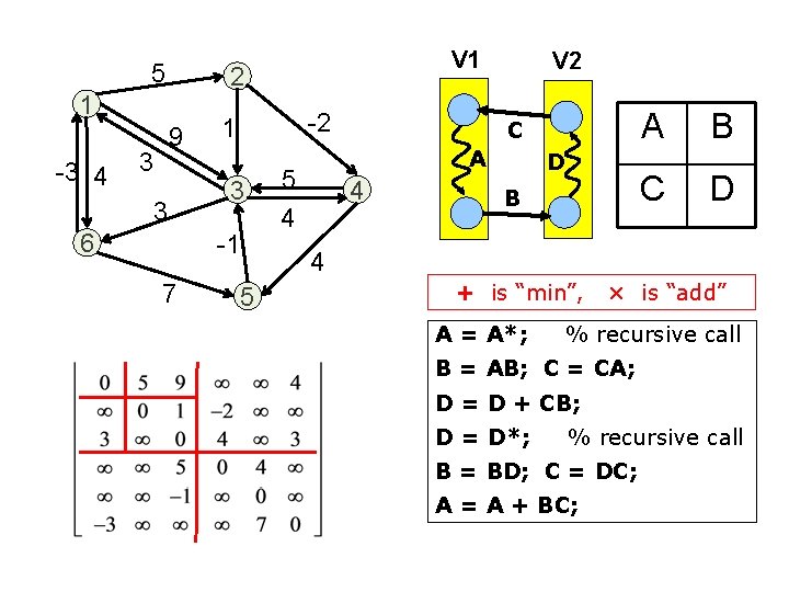
5 2 1 -3 4 9 3 V 1 3 6 -2 1 3 -1 7 V 2 C A 5 4 4 D B A B C D 4 5 + is “min”, A = A*; × is “add” % recursive call B = AB; C = CA; D = D + CB; D = D*; % recursive call B = BD; C = DC; A = A + BC;

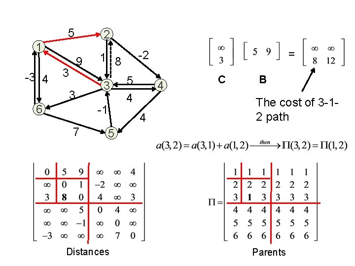
5 2 1 -3 4 9 3 3 6 3 -1 7 = -2 1 8 5 4 4 4 C B The cost of 3 -12 path 5 Distances Parents

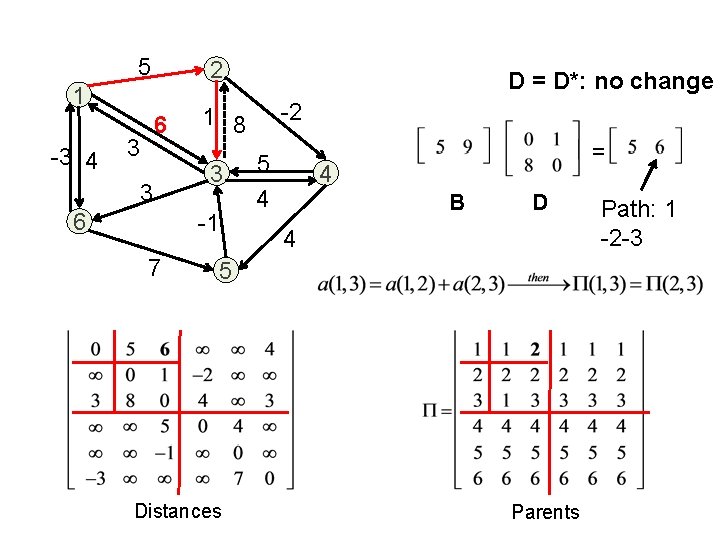
5 2 1 -3 4 6 3 3 6 -2 1 8 3 -1 7 D = D*: no change 5 4 = 4 B D 4 5 Distances Parents Path: 1 -2 -3

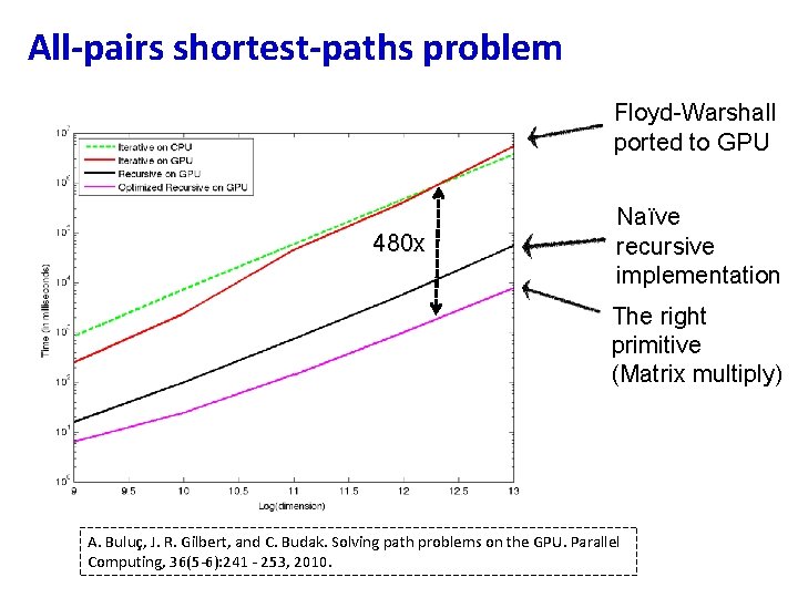
All-pairs shortest-paths problem Floyd-Warshall ported to GPU 480 x Naïve recursive implementation The right primitive (Matrix multiply) A. Buluç, J. R. Gilbert, and C. Budak. Solving path problems on the GPU. Parallel Computing, 36(5 -6): 241 - 253, 2010.

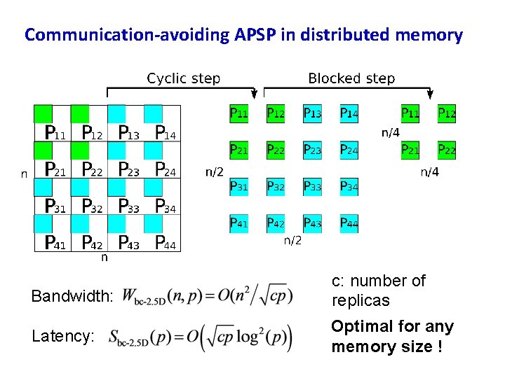
Communication-avoiding APSP in distributed memory Bandwidth: c: number of replicas Latency: Optimal for any memory size !

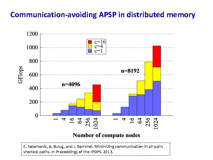
Communication-avoiding APSP in distributed memory E. Solomonik, A. Buluç, and J. Demmel. Minimizing communication in all-pairs shortest paths. In Proceedings of the IPDPS. 2013.

Lecture Outline • Applications • Designing parallel graph algorithms • Case studies: A. B. C. D. E. Graph traversals: Breadth-first search Shortest Paths: Delta-stepping, PHAST, Floyd-Warshall Ranking: Betweenness centrality Maximal Independent Sets: Luby’s algorithm Strongly Connected Components • Wrap-up: challenges on current systems

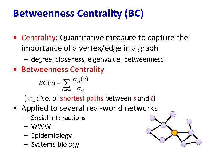
Betweenness Centrality (BC) • Centrality: Quantitative measure to capture the importance of a vertex/edge in a graph – degree, closeness, eigenvalue, betweenness • Betweenness Centrality ( : No. of shortest paths between s and t) • Applied to several real-world networks – – Social interactions WWW Epidemiology Systems biology

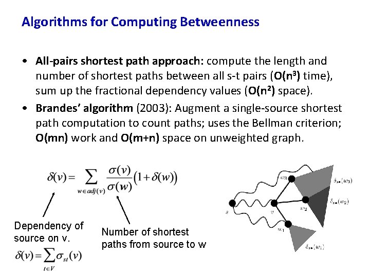
Algorithms for Computing Betweenness • All-pairs shortest path approach: compute the length and number of shortest paths between all s-t pairs (O(n 3) time), sum up the fractional dependency values (O(n 2) space). • Brandes’ algorithm (2003): Augment a single-source shortest path computation to count paths; uses the Bellman criterion; O(mn) work and O(m+n) space on unweighted graph. Dependency of source on v. Number of shortest paths from source to w

Parallel BC algorithms for unweighted graphs • High-level idea: Level-synchronous parallel breadthfirst search augmented to compute centrality scores • Two steps (both implemented as BFS) – traversal and path counting – dependency accumulation Shared-memory parallel algorithms for betweenness centrality Exact algorithm: O(mn) work, O(m+n) space, O(n. D+nm/p) time. D. A. Bader and K. Madduri. Parallel algorithms for evaluating centrality indices in real-world networks, ICPP’ 08 Improved with lower synchronization overhead and fewer noncontiguous memory references. K. Madduri, D. Ediger, K. Jiang, D. A. Bader, and D. Chavarria-Miranda. A faster parallel algorithm and efficient multithreaded implementations for evaluating betweenness centrality on massive datasets. MTAAP 2009

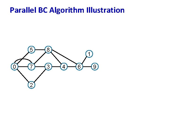
Parallel BC Algorithm Illustration 0 5 8 7 3 2 1 4 6 9

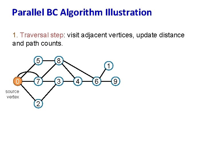
Parallel BC Algorithm Illustration 1. Traversal step: visit adjacent vertices, update distance and path counts. 0 5 8 7 3 source vertex 2 1 4 6 9

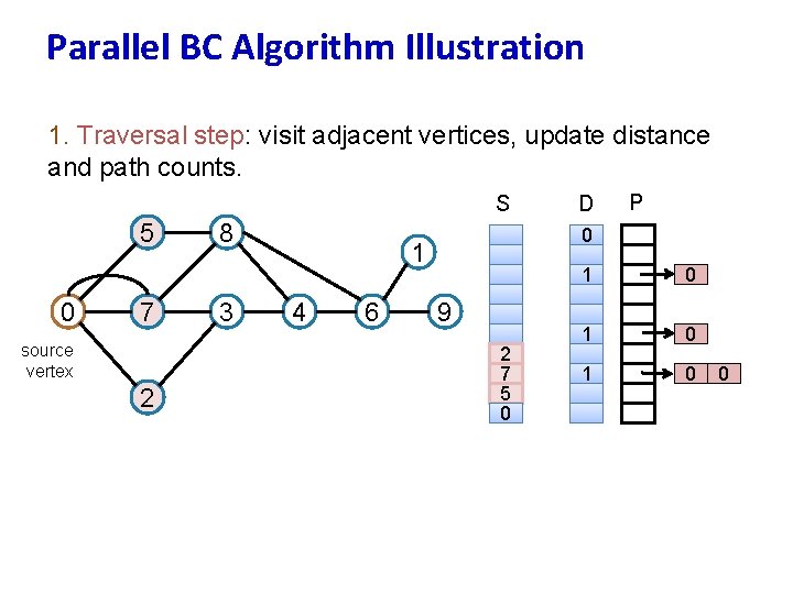
Parallel BC Algorithm Illustration 1. Traversal step: visit adjacent vertices, update distance and path counts. S 5 0 7 source vertex 2 8 3 6 P 0 1 4 D 9 2 7 5 0 1 0 1 0 0

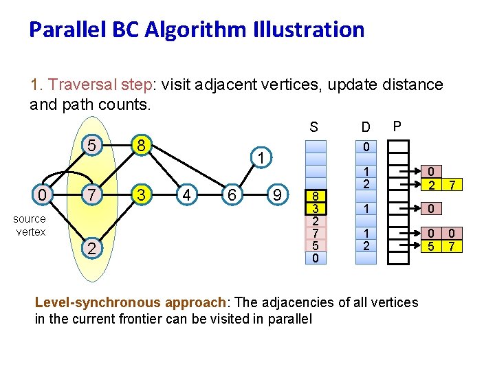
Parallel BC Algorithm Illustration 1. Traversal step: visit adjacent vertices, update distance and path counts. S 5 0 7 source vertex 2 8 3 6 P 0 1 4 D 9 8 3 2 7 5 0 1 2 0 2 1 0 1 2 0 5 Level-synchronous approach: The adjacencies of all vertices in the current frontier can be visited in parallel 7 0 7

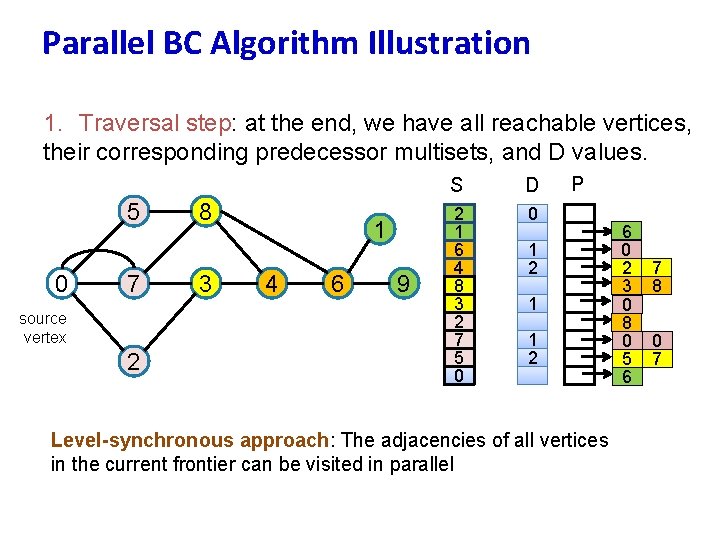
Parallel BC Algorithm Illustration 1. Traversal step: at the end, we have all reachable vertices, their corresponding predecessor multisets, and D values. 5 0 7 source vertex 2 8 3 1 4 6 9 S D 2 1 6 4 8 3 2 7 5 0 0 P 1 2 1 1 2 Level-synchronous approach: The adjacencies of all vertices in the current frontier can be visited in parallel 6 0 2 3 0 8 0 5 6 7 8 0 7

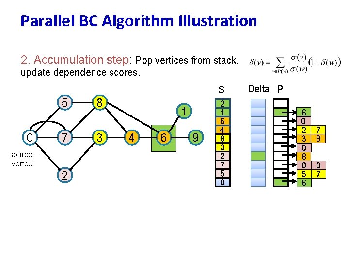
Parallel BC Algorithm Illustration 2. Accumulation step: Pop vertices from stack, update dependence scores. S 5 0 7 source vertex 2 8 3 1 4 6 9 2 1 6 4 8 3 2 7 5 0 Delta P 6 0 2 3 0 8 0 5 6 7 8 0 7

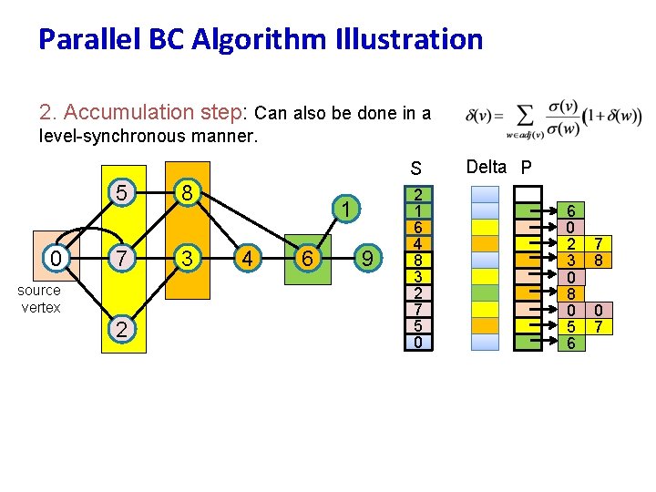
Parallel BC Algorithm Illustration 2. Accumulation step: Can also be done in a level-synchronous manner. S 5 0 7 source vertex 2 8 3 1 4 6 9 2 1 6 4 8 3 2 7 5 0 Delta P 6 0 2 3 0 8 0 5 6 7 8 0 7

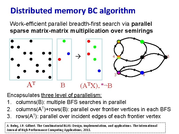
Distributed memory BC algorithm Work-efficient parallel breadth-first search via parallel sparse matrix-matrix multiplication over semirings 4 3 AT B 7 5 6 . (ATX) *¬B Encapsulates three level of parallelism: 1. columns(B): multiple BFS searches in parallel 2. columns(AT)+rows(B): parallel over frontier vertices in each BFS 3. rows(AT): parallel over incident edges of each frontier vertex A. Buluç, J. R. Gilbert. The Combinatorial BLAS: Design, implementation, and applications. The International Journal of High Performance Computing Applications, 2011.

Lecture Outline • Applications • Designing parallel graph algorithms • Case studies: A. B. C. D. E. Graph traversals: Breadth-first search Shortest Paths: Delta-stepping, PHAST, Floyd-Warshall Ranking: Betweenness centrality Maximal Independent Sets: Luby’s algorithm Strongly Connected Components • Wrap-up: challenges on current systems

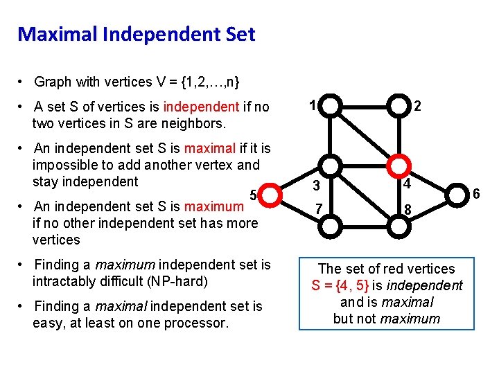
Maximal Independent Set • Graph with vertices V = {1, 2, …, n} • A set S of vertices is independent if no two vertices in S are neighbors. • An independent set S is maximal if it is impossible to add another vertex and stay independent 5 • An independent set S is maximum if no other independent set has more vertices • Finding a maximum independent set is intractably difficult (NP-hard) • Finding a maximal independent set is easy, at least on one processor. 1 2 3 4 7 8 The set of red vertices S = {4, 5} is independent and is maximal but not maximum 6

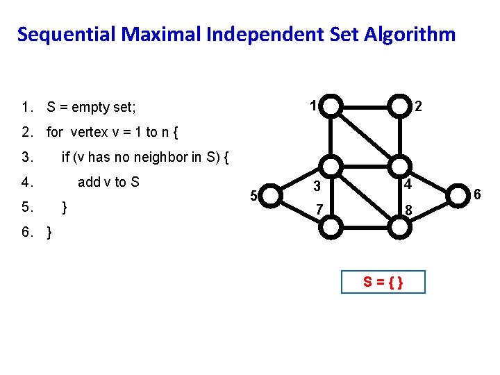
Sequential Maximal Independent Set Algorithm 1 1. S = empty set; 2 2. for vertex v = 1 to n { 3. if (v has no neighbor in S) { 4. 5. add v to S } 5 3 4 7 8 6. } S={} 6

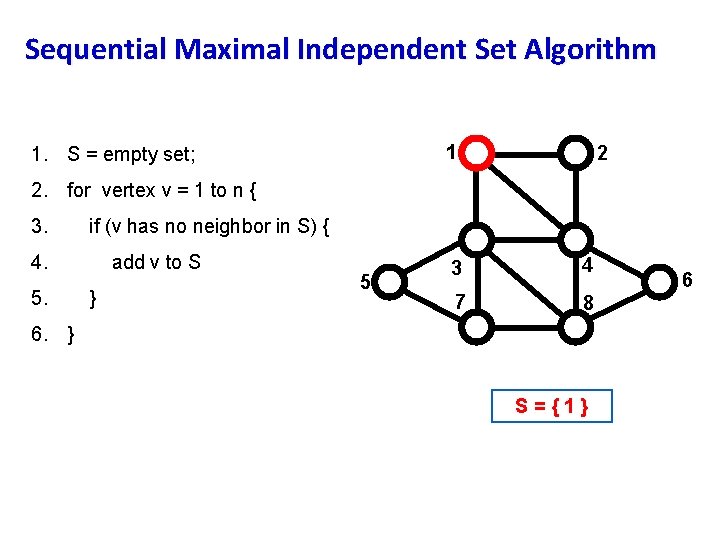
Sequential Maximal Independent Set Algorithm 1 1. S = empty set; 2 2. for vertex v = 1 to n { 3. if (v has no neighbor in S) { 4. 5. add v to S } 5 3 4 7 8 6. } S={1} 6

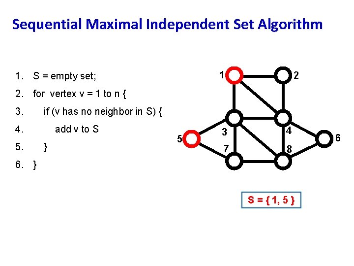
Sequential Maximal Independent Set Algorithm 1 1. S = empty set; 2 2. for vertex v = 1 to n { 3. if (v has no neighbor in S) { 4. 5. add v to S } 5 3 4 7 8 6. } S = { 1, 5 } 6

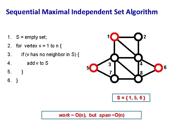
Sequential Maximal Independent Set Algorithm 1 1. S = empty set; 2 2. for vertex v = 1 to n { 3. if (v has no neighbor in S) { 4. 5. add v to S } 5 3 4 7 8 6. } S = { 1, 5, 6 } work ~ O(n), but span ~O(n) 6

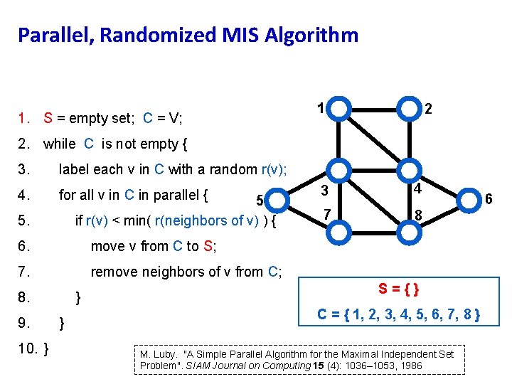
Parallel, Randomized MIS Algorithm 1. S = empty set; C = V; 1 2 2. while C is not empty { 3. label each v in C with a random r(v); 4. for all v in C in parallel { 5 if r(v) < min( r(neighbors of v) ) { 5. 6. move v from C to S; 7. remove neighbors of v from C; 8. 9. 10. } } } 3 4 7 8 S={} C = { 1, 2, 3, 4, 5, 6, 7, 8 } M. Luby. "A Simple Parallel Algorithm for the Maximal Independent Set Problem". SIAM Journal on Computing 15 (4): 1036– 1053, 1986 6

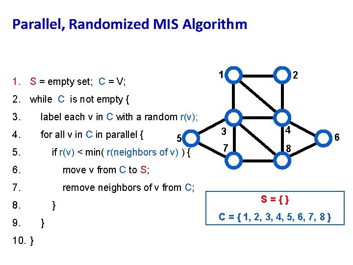
Parallel, Randomized MIS Algorithm 1. S = empty set; C = V; 1 2 2. while C is not empty { 3. label each v in C with a random r(v); 4. for all v in C in parallel { 5 if r(v) < min( r(neighbors of v) ) { 5. 6. move v from C to S; 7. remove neighbors of v from C; 8. 9. 10. } } } 3 4 7 8 S={} C = { 1, 2, 3, 4, 5, 6, 7, 8 } 6

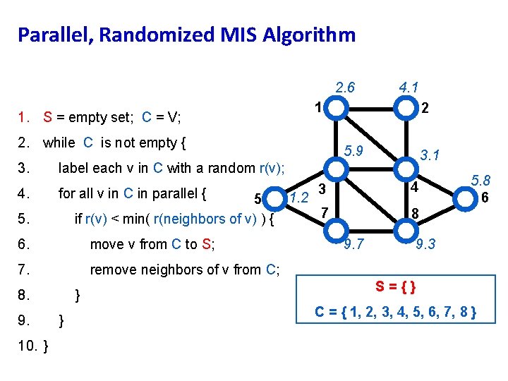
Parallel, Randomized MIS Algorithm 2. 6 1 1. S = empty set; C = V; 2. while C is not empty { 3. 4. for all v in C in parallel { 5 if r(v) < min( r(neighbors of v) ) { 6. move v from C to S; 7. remove neighbors of v from C; 8. 10. } 2 5. 9 3. 1 label each v in C with a random r(v); 5. 9. 4. 1 } } 1. 2 3 4 7 8 9. 7 5. 8 6 9. 3 S={} C = { 1, 2, 3, 4, 5, 6, 7, 8 }

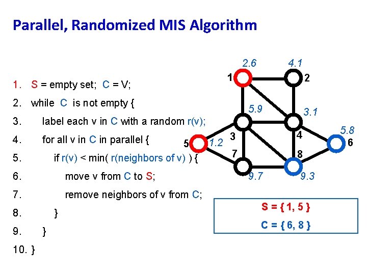
Parallel, Randomized MIS Algorithm 2. 6 1 1. S = empty set; C = V; 2. while C is not empty { 3. 4. for all v in C in parallel { 5 if r(v) < min( r(neighbors of v) ) { 6. move v from C to S; 7. remove neighbors of v from C; 8. 10. } 2 5. 9 3. 1 label each v in C with a random r(v); 5. 9. 4. 1 } } 1. 2 3 4 7 8 9. 7 9. 3 S = { 1, 5 } C = { 6, 8 } 5. 8 6

Parallel, Randomized MIS Algorithm 1. S = empty set; C = V; 1 2 2. while C is not empty { 3. 4. label each v in C with a random r(v); for all v in C in parallel { 5 if r(v) < min( r(neighbors of v) ) { 5. 6. move v from C to S; 7. remove neighbors of v from C; 8. 9. 10. } } } 3 4 7 8 1. 8 S = { 1, 5 } C = { 6, 8 } 2. 7 6

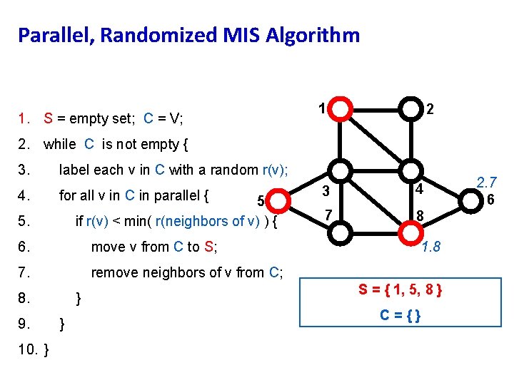
Parallel, Randomized MIS Algorithm 1. S = empty set; C = V; 1 2 2. while C is not empty { 3. 4. label each v in C with a random r(v); for all v in C in parallel { 5 if r(v) < min( r(neighbors of v) ) { 5. 6. move v from C to S; 7. remove neighbors of v from C; 8. 9. 10. } } } 3 4 7 8 1. 8 S = { 1, 5, 8 } C={} 2. 7 6

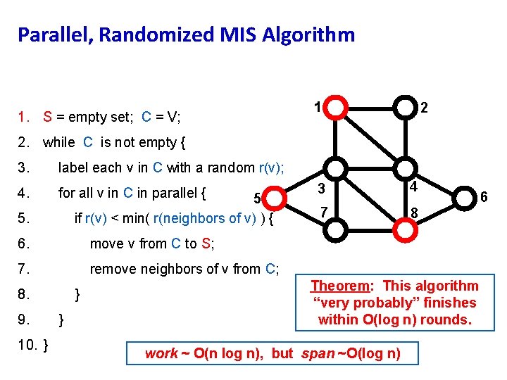
Parallel, Randomized MIS Algorithm 1. S = empty set; C = V; 1 2 2. while C is not empty { 3. label each v in C with a random r(v); 4. for all v in C in parallel { 5 if r(v) < min( r(neighbors of v) ) { 5. 6. move v from C to S; 7. remove neighbors of v from C; 8. 9. 10. } } } 3 4 7 8 Theorem: This algorithm “very probably” finishes within O(log n) rounds. work ~ O(n log n), but span ~O(log n) 6

Lecture Outline • Applications • Designing parallel graph algorithms • Case studies: A. B. C. D. E. Graph traversals: Breadth-first search Shortest Paths: Delta-stepping, PHAST, Floyd-Warshall Ranking: Betweenness centrality Maximal Independent Sets: Luby’s algorithm Strongly Connected Components • Wrap-up: challenges on current systems

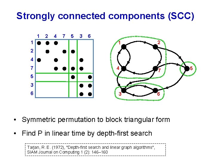
Strongly connected components (SCC) 1 1 2 4 7 5 3 6 1 2 2 4 7 5 3 6 • Symmetric permutation to block triangular form • Find P in linear time by depth-first search Tarjan, R. E. (1972), "Depth-first search and linear graph algorithms", SIAM Journal on Computing 1 (2): 146– 160 5

Strongly connected components of directed graph • Sequential: use depth-first search (Tarjan); work=O(m+n) for m=|E|, n=|V|. • DFS seems to be inherently sequential. • Parallel: divide-and-conquer and BFS (Fleischer et al. ); worst-case span O(n) but good in practice on many graphs. L. Fleischer, B. Hendrickson, and A. Pınar. On identifying strongly connected components in parallel. Parallel and Distributed Processing, pages 505– 511, 2000.

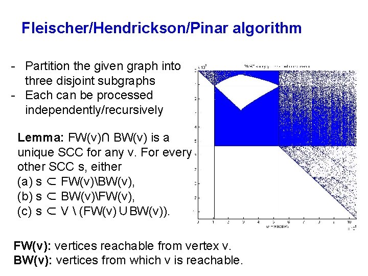
Fleischer/Hendrickson/Pinar algorithm - Partition the given graph into three disjoint subgraphs - Each can be processed independently/recursively Lemma: FW(v)∩ BW(v) is a unique SCC for any v. For every other SCC s, either (a) s ⊂ FW(v)BW(v), (b) s ⊂ BW(v)FW(v), (c) s ⊂ V (FW(v)∪BW(v)). FW(v): vertices reachable from vertex v. BW(v): vertices from which v is reachable.

Lecture Outline • Applications • Designing parallel graph algorithms • Case studies: A. B. C. D. E. Graph traversals: Breadth-first search Shortest Paths: Delta-stepping, PHAST, Floyd-Warshall Ranking: Betweenness centrality Maximal Independent Sets: Luby’s algorithm Strongly Connected Components • Wrap-up: challenges on current systems

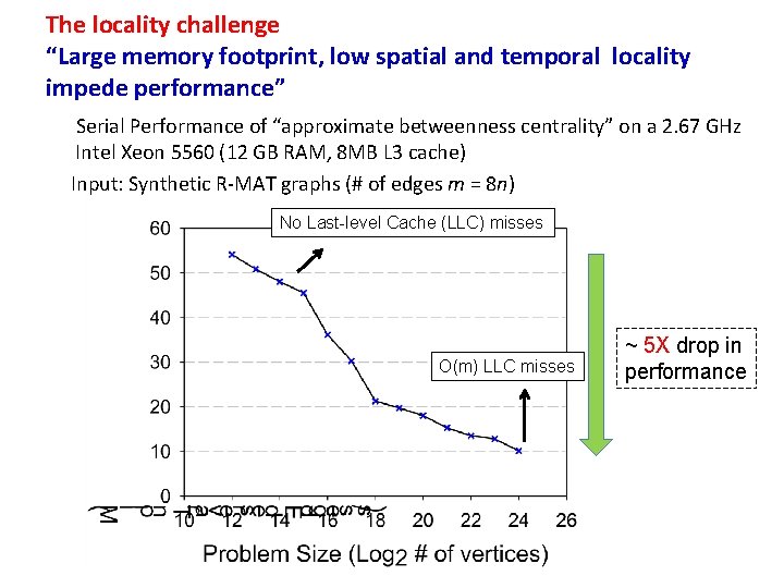
The locality challenge “Large memory footprint, low spatial and temporal locality impede performance” Serial Performance of “approximate betweenness centrality” on a 2. 67 GHz Intel Xeon 5560 (12 GB RAM, 8 MB L 3 cache) Input: Synthetic R-MAT graphs (# of edges m = 8 n) No Last-level Cache (LLC) misses O(m) LLC misses ~ 5 X drop in performance

The parallel scaling challenge “Classical parallel graph algorithms perform poorly on current parallel systems” • Graph topology assumptions in classical algorithms do not match real-world datasets • Parallelization strategies at loggerheads with techniques for enhancing memory locality • Classical “work-efficient” graph algorithms may not fully exploit new architectural features – Increasing complexity of memory hierarchy, processor heterogeneity, wide SIMD. • Tuning implementation to minimize parallel overhead is nontrivial – Shared memory: minimizing overhead of locks, barriers. – Distributed memory: bounding message buffer sizes, bundling messages, overlapping communication w/ computation.

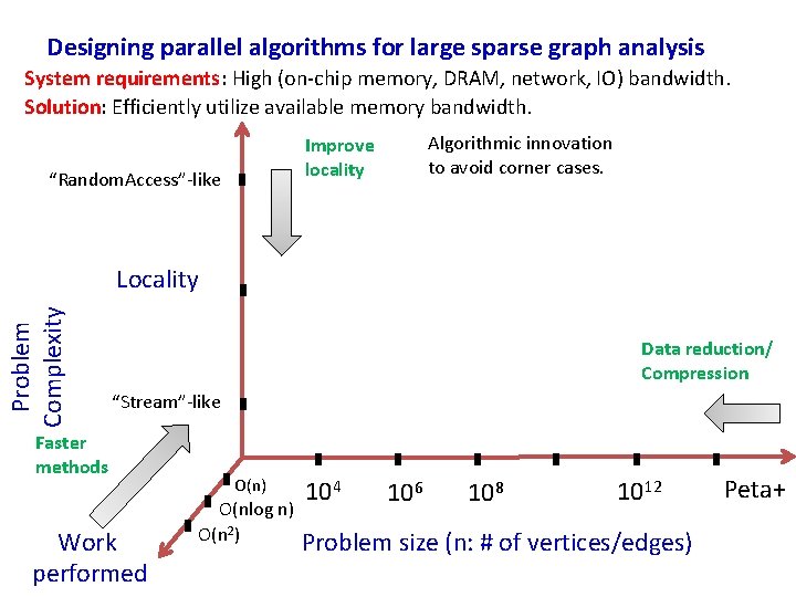
Designing parallel algorithms for large sparse graph analysis System requirements: High (on-chip memory, DRAM, network, IO) bandwidth. Solution: Efficiently utilize available memory bandwidth. Algorithmic innovation to avoid corner cases. Improve locality “Random. Access”-like Problem Complexity Locality Data reduction/ Compression “Stream”-like Faster methods Work performed O(n) O(nlog n) O(n 2) 104 106 108 1012 Problem size (n: # of vertices/edges) Peta+

Conclusions • Best algorithm depends on the input. • Communication costs (and hence data distribution) is crucial for distributed memory. • Locality is crucial for in-node performance. • Graph traversal (BFS) is fundamental building block for more complex algorithms. • Best parallel algorithm can be significantly different than the best serial algorithm.