Parallel GPU computing in MATLAB ITS Research Computing

Parallel & GPU computing in MATLAB ITS Research Computing Mark Reed markreed@unc. edu

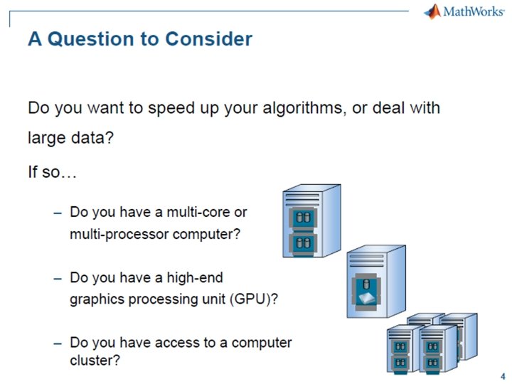
Objectives • Introductory level MATLAB course for people who want to learn parallel or GPU computing in MATLAB. • Help participants determine when to use parallel computing and how to use MATLAB parallel & GPU computing on their local computer & on the Research Computing clusters

Logistics • Course Format • Overview of MATLAB topics with Lab Exercises • UNC Research Computing Ø http: //its. unc. edu/research

Agenda • Parallel computing Ø Ø Ø What is it? Why use it? How to write MATLAB code in parallel • GPU computing Ø What is it & why use it? Ø How to write MATLAB code in for GPU computing • How to run MATLAB parallel & GPU code on the UNC cluster Ø Quick introduction to the UNC clusters (Dogwood, Longleaf) sbatch commands and what they mean • Questions Ø

Parallel Computing

What is Parallel Computing? • Parallel Computing: Using multiple computer processing units (CPUs) to solve a problem at the same time • The compute resources might be: computer with multiple processors or networked computers Source: https: //computing. llnl. gov/tutorials/parallel_comp/

Parallel Code • Why? Ø Ø Faster time to solution Solve bigger problems • The computational problem should be able to: Ø Ø Be broken into discrete parts that can be solved simultaneously and independently Be solved in less time with multiple compute resources than with a single compute resource.

Parallel Computing in MATLAB

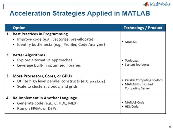
3 Levels of Parallel Computing • Built-in multithreading Ø shared memory, single node • Parallel Computing Toolbox (PCT) Ø Ø shared memory, single node parfor • Matlab Distributed Computing Server (MDCS) Ø Ø distributed computing across nodes spmd or parfor

Built-in Multithreading • Operations in the algorithm carried out by the function are easily partitioned into sections that can be executed concurrently, and with little communication or few sequential operations required. • Data size is large enough so that any advantages of concurrent execution outweigh the time required to partition the data and manage separate execution threads. For example, most functions speed up only when the array is greater than several thousand elements. • Operation is not memory-bound where the processing time is dominated by memory access time. As a general rule, more complex functions speed up better than simple functions. • http: //www. mathworks. com/matlabcentral/answers/95958 -which-matlabfunctions-benefit-from-multithreaded-computation

Built-in Multithreading • Easiest to use but least effective. • Interferes with other users jobs when run in a shared environment unless you know what you are doing • -single. Comp. Thread option disables this (RC wrapper scripts set this option!) • Use the function max. Num. Comp. Threads to set the number of threads (default is all of them) • Make sure to submit using –n option to match max. Num. Comp. Threads and set “–N 1”

Multithreading solving linear system of equations: y=A*b • Sample scaling, run on Matlab 2013 a size=10000, time=0. 071195, threads=1, speedup=1. 000000, efficiency=100. 000000 % size=10000, time=0. 034743, threads=2, speedup=2. 049190, efficiency=102. 459488 % size=10000, time=0. 023221, threads=4, speedup=3. 065975, efficiency=76. 649369 % size=10000, time=0. 024257, threads=8, speedup=2. 935029, efficiency=36. 687863 % size=10000, time=0. 023156, threads=12, speedup=3. 074581, efficiency=25. 621509 % size=40000, time=1. 133684, threads=1, speedup=1. 000000, efficiency=100. 000000 % size=40000, time=0. 609896, threads=2, speedup=1. 858815, efficiency=92. 940764 % size=40000, time=0. 384364, threads=4, speedup=2. 949506, efficiency=73. 737655 % size=40000, time=0. 354435, threads=8, speedup=3. 198567, efficiency=39. 982084 % size=40000, time=0. 341615, threads=12, speedup=3. 318601, efficiency=27. 655011 % size=50000, time=1. 779888, threads=1, speedup=1. 000000, efficiency=100. 000000 % size=50000, time=0. 964425, threads=2, speedup=1. 845543, efficiency=92. 277160 % size=50000, time=0. 616930, threads=4, speedup=2. 885073, efficiency=72. 126822 % size=50000, time=0. 543360, threads=8, speedup=3. 275707, efficiency=40. 946334 % size=50000, time=0. 532957, threads=12, speedup=3. 339647, efficiency=27. 830388 %

Matrix Multiply code from implicit multithreading example % create a list of thread counts and sizes, then loop over sizes nthreads = { 1, 2, 4, 8, 12 }; sizes = [1000 2000 4000]; for s=1: 3 n = sizes(s); % set matrix size A = rand(n); % create random matrix B = rand(n); % create another random matrix for i=1: 5 % vector implementation (may trigger multithreading) nt=nthreads{i}; lastnt=max. Num. Comp. Threads(nt); % set the thread count tic % starts timer C = A * B; % matrix multiplication walltime(i) = toc; % wall clock time Speedup = walltime(1)/walltime(i); Efficiency = 100*Speedup/nt; printstring=sprintf (['size=%d time=%8. 4 f threads=%2 d speedup=%4. 1 f efficiency=%5. 1 f %%'], n, walltime(i), nt, Speedup, Efficiency); disp(printstring); end disp(' '); end % end for size j

Multithreading matrix multiply: C=A*B size=1000 size=1000 time= time= 0. 1893 0. 0946 0. 0494 0. 0261 0. 0235 threads= 1 speedup= 1. 0 efficiency=100. 0 % threads= 2 speedup= 2. 0 efficiency=100. 0 % threads= 4 speedup= 3. 8 efficiency= 95. 8 % threads= 8 speedup= 7. 3 efficiency= 90. 8 % threads=12 speedup= 8. 1 efficiency= 67. 2 % size=2000 size=2000 time= time= 1. 4376 0. 7297 0. 3731 0. 1946 0. 1349 threads= 1 speedup= 1. 0 efficiency=100. 0 % threads= 2 speedup= 2. 0 efficiency= 98. 5 % threads= 4 speedup= 3. 9 efficiency= 96. 3 % threads= 8 speedup= 7. 4 efficiency= 92. 3 % threads=12 speedup=10. 7 efficiency= 88. 8 % size=4000 size=4000 time= 11. 4206 threads= 1 speedup= 1. 0 efficiency=100. 0 % time= 5. 7619 threads= 2 speedup= 2. 0 efficiency= 99. 1 % time= 2. 9057 threads= 4 speedup= 3. 9 efficiency= 98. 3 % time= 1. 4557 threads= 8 speedup= 7. 8 efficiency= 98. 1 % time= 1. 0311 threads=12 speedup=11. 1 efficiency= 92. 3 % YMMV. Some work better than others!

Parallel Computing in MATLAB • MATLAB Parallel Computing Toolbox (available for use at UNC) Ø Ø Workers limited only by resources on the node, see parallel preferences for the default. Typically the entire node. Built in functions for parallel computing § parfor loop (for running task-parallel algorithms on multiple processors) § spmd (handles large datasets and data-parallel algorithms)

Matlab Distributed Computing Toolbox • Allows MATLAB to run as many workers on a remote cluster of computers as licensing allows. Ø Ø Re. Co has 256 licenses A single user can check out up to 64 (this will be changed for Dogwood) • Note the key word “distributed” meaning it will run between nodes

Primary Parallel Commands • parpool (prior to Matlab 2013 b this was parpool) Ø Ø Ø mypool = parpool(4) … do work … delete(mypool) • parfor (for loop) • spmd (distributed computing for datasets)

parpool • Use parpool to open a pool of “workers” to execute code on other compute cores. • In Matlab parlance these are called workers, think of them like threads or processes • You can open these workers locally (on the same node) or remotely • Local access is enabled by the Parallel Computing Toolkit, remote access is enabled via MDCS (Matlab Distributed Computing Server)

Starting a parpool • mypool = parpool (‘local’, 4); • Mypool = parpool(4); Ø Ø Opens 4 workers locally on the same node Communication is fastest within a node Make sure you submitted your Matlab job with “-n X” where X matches the number of workers you open!!! And use –N 1 to ensure the slots are all on the same node (i. e. local) • Use display(mypool) to show information about the pool

Closing a parallel pool • Use delete(mypool) to end parallel session • If you didn’t save the name you can use Ø delete (gcp(‘nocreate’));

Parallel for Loops (parfor) • parfor loops can execute for loop like code in parallel to significantly improve performance • Must consist of code broken into discrete parts that can be solved simultaneously, each iteration is independent (task independent) • No guaranteed order of iterations Ø i. e. order independent • Scalar values defined outside of the loop but used inside of it are broadcast to all workers

Parfor example Will work in parallel, loop increments are not dependent on each other: mypool =parpool(2) j=zeros(100, 1); %pre-allocate vector parfor i=1: 100; Makes the loop j(i, 1)=5*i; run in parallel end; delete (mypool);

Serial Loop example • Won’t work in parallel- it’s serial: j=zeros(100, 1); %pre-allocate vector j(1)=5; j(i-1) for i=2: 100; needed to j(i, 1)=j(i-1)+5; calculate end; j(i, 1) serial!!!

Classifying Variables in parfor Loop • A parfor-loop variable is classified into one of several categories. A parfor-loop generates an error if it contains any variables that cannot be uniquely categorized or if any variables violate their category restrictions.

Parfor Loop Variables • Loop Variables Ø Loop index • Sliced Variables Ø Arrays whose segments are operated on by different iterations of the loop • Broadcast Variables Ø Ø Variables defined before the loop whose value is required inside the loop, but never assigned inside the loop. Consider whether it is faster to create them on workers • Reduction Variables Ø Variables that accumulate a value across iterations of the loop, regardless of iteration order • Temporary Variables Ø Variables that accumulate a value across iterations of the loop, regardless of iteration order

Parfor Variable Types - Example https: //www. mathworks. com/help/distcomp/classification-ofvariables-in-parfor-loops. html

Constraints • The loop variable cannot be used to index with other variables • No inter-process communication. Therefore, a parfor loop cannot contain: Ø Ø break and return statements global and persistent variables nested functions changes to handle classes • Transparency Ø Ø Cannot “introduce” variables (e. g. eval, load, global, etc. ) Unambiguous Variables Names • No nested parfor loops or spmd statement Slide from Raymond Norris, Mathworks

Parallel for Loops (parfor) • There is overhead in creating workers and partitioning work to them, and collecting work from them • Loops need to be computationally intensive to offset this overhead

Test the efficiency of your parallel code • Use MATLAB’s tic & toc functions Ø Ø Tic starts a timer Toc tells you the number of seconds since the tic function was called

Tic & Toc Simple Example tic; parfor i=1: 10 z(i)=10; end; toc

rand in parfor loops • MATLAB has a repeatable sequence of random numbers • When workers are started up, rather than using this same sequence of random numbers, the labindex is used to seed the RNG

spmd • Single Program Multiple Data model • Used to create parallel regions of code • Values returning from the body of an spmd statement are converted to Composite objects • A Composite object contains references to the values stored on the remote MATLAB workers, and those values can be retrieved using cell-array indexing. • The actual data on the workers remains available on the workers for subsequent spmd execution, so long as the Composite exists on the client and the parallel pool remains open.

spmd • spmd distributes the array among MATLAB workers (each worker contains a part of the array) but can still operate on entire array as 1 entity • Inside the body of the spmd statement, each MATLAB worker has a unique value of labindex, while numlabs denotes the total number of workers executing the block in parallel. • Data automatically transferred between workers when necessary • Within the body of the spmd statement, communication functions for communicating jobs (such as lab. Send and lab. Receive) can transfer data between the workers.

Spmd Format • Format • Simple Example parpool (4) spmd statements end parpool(4) spmd j=zeros(1 e 7, 1); end;

Spmd Examples • Result j is a Composite with 4 parts!

MATLAB Composites • Its an object used for data distribution in MATLAB • A Composite object has one entry for each worker Ø Ø parpool(12) creates? parpool(6) creates? 12 X 1 composite 6 X 1 composite

MATLAB Composites • You can create a composite in two ways: Ø Ø spmd c = Composite(); § This creates a composite that does not contain any data, just placeholders for data § Also, one element per parpool worker is created for the composite § Use smpd or indexing to populate a composite created this way

Another spmd Example- creating graphs %Perform a simple calculation in parallel, and plot the results: parpool(4) spmd % build magic squares in parallel q = magic(labindex + 2); %labindex- index of the lab/worker (e. g. 1) end for ii=1: length(q) % plot each magic square figure, imagesc(q{ii}); %plot a matrix as an image end delete (gcp(‘nocreate’));

Another spmd Example- creating graphs • Results

spmd vs parfor • • parfor is simpler to use parfor can’t control iterations parfor only does loops spmd more control over iterations spmd more control over data movement spmd is persistent spmd is more flexible and you can create parallel regions that do more than just loop

GPU Computing

What is GPU computing? • GPU computing is the use of a GPU (graphics processing unit) with a CPU to accelerate performance • Offloads compute-intensive portions an application to the GPU, and remainder of code runs on CPU

What is GPU computing? • CPUs consist of a few cores optimized for serial processing. • GPUs consist of thousands of smaller cores designed for parallel performance (i. e. more memory bandwidth and cores) • Data is moved between CPU Main Memory and GPU Device Memory via the PCIe Bus

GPU Computing PCIe Bus

What/Why GPU computing? • Serial portions of the code run on the CPU while parallel portions run on the GPU • From a user's perspective, applications in general run significantly faster

Write GPU computing codes in MATLAB • Transfer data between the MATLAB workspace & the GPU Ø Accomplished by a GPUArray § Data stored on the GPU. Ø Use gpu. Array function to transfer an array from the MATLAB workspace to the GPU

Write GPU computing codes in MATLAB • Examples N = 6; M = magic(N); G = gpu. Array(M); %create array stored on GPU • G is a MATLAB GPUArray object representing magic square data on the GPU. X = rand(1000); G = gpu. Array(X); %array stored on GPU

Static GPUArrays • Static GPUArrays allow users to directly construct arrays on GPUs, without transfers • Include:

Static Array Examples • Construct an Identity Matrix on the GPU II = parallel. gpu. GPUArray. eye(1024, 'int 32'); size(II) 1024 • Construct a Multidimensional Array on the GPU G = parallel. gpu. GPUArray. ones(100, 50); size(G) 100 50 class. Underlying(G) Double %double is default, so don’t need to specify it

More Resources for GPU Arrays • For a complete list of available static methods in any release, type methods('parallel. gpu. GPUArray') • For help on any one of the constructors, type help parallel. gpu. GPUArray/functionname • For example, to see the help on the colon constructor, type help parallel. gpu. GPUArray/colon

Retrieve Data from the GPU • Use gather function Ø Makes data available in GPU environment, available in MATLAB workspace (CPU) • Example G = gpu. Array(ones(100, 'uint 32')); %array stored only on GPU D = gather(G); %bring D to CPU/MATLAB workspace OK = isequal(D, ones(100, 'uint 32')) %check to see if the array on the GPU is the same as the array brought to the CPU

Calling Functions with GPU Objects • Example uses the fft and real functions, arithmetic operators + and *. • Calculations are performed on the GPU, gather retrieves data from the GPU to workspace. Ga = gpu. Array(rand(1000, 'single')); %array on GPU & next operations performed on GPU Gfft = fft(Ga); Gb = (real(Gfft) + Ga) * 6; G = gather(Gb); brings G to the CPU

Calling Functions with GPU Objects • The whos command is instructive for showing where each variable's data is stored. whos Name Size Bytes Class G 1000 x 1000 4000000 single Ga 1000 x 1000 108 parallel. gpu. GPUArray Gb 1000 x 1000 108 parallel. gpu. GPUArray Gfft 1000 x 1000 108 parallel. gpu. GPUArray • All arrays are stored on the GPU (GPUArray), except G, because it was “gathered”

2 D Wave Equation Example Highlights are the only differences between GPU and regular code function vvg = Wave. GPU(N, Nsteps) % From http: //blogs. mathworks. com/loren/2012/02/06/using-gpus-in-matlab/ % %% Solving 2 nd Order Wave Equation Using Spectral Methods % This example solves a 2 nd order wave equation: utt = uxx + uyy, with u = % 0 on the boundaries. It uses a 2 nd order central finite difference in % time and a Chebysehv spectral method in space (using FFT). % % The code has been modified from an example in Spectral Methods in MATLAB % by Trefethen, Lloyd N. % Points in X and Y x = cos(pi*(0: N)/N); % using Chebyshev points % Send x to the GPU x = gpu. Array(x); y = x'; % Calculating time step dt = 6/N^2;

2 D Wave Example Cont. % Setting up grid [xx, yy] = meshgrid(x, y); % Calculate initial values vv = exp(-40*((xx-. 4). ^2 + yy. ^2)); vvold = vv; ii = 2: N; index 1 = 1 i*[0: N-1 0 1 -N: -1]; index 2 = -[0: N 1 -N: -1]. ^2; % Sending data to the GPU dt = gpu. Array(dt); index 1 = gpu. Array(index 1); index 2 = gpu. Array(index 2); % Creating weights used for spectral differentiation W 1 T = repmat(index 1, N-1, 1); W 2 T = repmat(index 2, N-1, 1); W 3 T = repmat(index 1. ', 1, N-1); W 4 T = repmat(index 2. ', 1, N-1); Wuxx. T 1 = repmat((1. /(1 -x(ii). ^2)), N-1, 1); Wuxx. T 2 = repmat(x(ii). /(1 -x(ii). ^2). ^(3/2), N-1, 1); Wuyy. T 1 = repmat(1. /(1 -y(ii). ^2), 1, N-1); Wuyy. T 2 = repmat(y(ii). /(1 -y(ii). ^2). ^(3/2), 1, N-1); % Start time-stepping n = 0; while n < Nsteps [vv, vvold] = stepsolution(vv, vvold, ii, N, dt, W 1 T, W 2 T, W 3 T, W 4 T, . . . Wuxx. T 1, Wuxx. T 2, Wuyy. T 1, Wuyy. T 2); n = n + 1; end % Gather vvg back from GPU memory when done vvg = gather(vv);

Running Functions on GPU • Call arrayfun with a function handle to the MATLAB function as the first input argument: result = arrayfun(@my. Function, arg 1, arg 2); • Subsequent arguments provide inputs to the MATLAB function. • Input arguments can be workspace data or GPUArray. Ø Ø GPUArray type input arguments return GPUArray. Else arrayfun executes in the CPU

Running Functions on GPU Example: function applies correction to an array function c = my. Cal(rawdata, gain, offset) c = (rawdata. * gain) + offset; • Function performs only element-wise operations when applying a gain factor and offset to each element of the rawdata array.

Running Functions on GPU • Create some nominal measurement: meas = ones(1000)*3; % 1000 -by-1000 matrix • Function allows the gain and offset to be arrays of the same size as rawdata, so unique corrections can be applied to individual measurements. • Typically keep the correction data on the GPU so you do not have to transfer it for each application:

Running Functions on GPU % Runs on the GPU because the input arguments % gn and offs are in GPU memory; gn = gpu. Array(rand(1000))/100 + 0. 995; offs = gpu. Array(rand(1000))/50 - 0. 01; corrected = arrayfun(@my. Cal, meas, gn, offs); % Retrieve the corrected results from the GPU to % the MATLAB workspace; results = gather(corrected);

Identify & Select GPU • If you have only one GPU in your computer, that GPU is the default. • If you have more than one GPU card in your computer, you can use the following functions to identify and select which card you want to use:

Identify & Select GPU • This example shows how to identify and GPU a for your computations Ø First, determine the number of GPU devices on your computer using gpu. Device. Count

Identify & Select GPU • In this case, you have 2 devices, thus the first is the default. Ø Ø To examine it’s properties type gpu. Device Output from Killdevil

Identify & Select GPU • If the previous GPU is the device you want to use, then you can just proceed with the default • To use another device call gpu. Device with the index of the card and view its properties to verify you want to use it. Here is an example where the second device is chosen

More Resources for GPU computing • MATLAB’s extensive online help documents for GPU computing Ø http: //www. mathworks. com/help/toolbox/distco mp/bsic 3 by. html

Parallel & GPU Computing on the cluster

Cluster Jargon • Node Ø A standalone "computer in a box". Usually comprised of multiple CPUs/processors/cores. Nodes are networked together to comprise a cluster. • Nodes have two sockets (CPUs) each of which runs multiple cores (e. g. most Longleaf nodes have 12 cores per socket, i. e. 24 per node). Hyper-threading turned on doubles this number. • Each thread can run a process

Using MATLAB on the computer Cluster • What? ? Ø UNC provides researchers and graduate students with access to extremely powerful computers to use for their research. Ø Longleaf is a Linux based computing system with > 5000 cores Ø Killdevil is a Linux based computing system with ~ 9500 cores • Why? ? Ø The cluster is an extremely fast and efficient way to run LARGE MATLAB programs (fewer “Out of Memory” errors!) Ø You can get more done! Your programs run on the cluster which frees your computer for writing and debugging other programs!!! Ø You can run a large number at the same time

Using MATLAB on the computer Cluster • Where and When? ? Ø The cluster is available 24/7 and you can run programs remotely from anywhere with an internet connection!

Using MATLAB on the computer Cluster • Overview of how to use the computer cluster Ø It would be helpful to take the following courses: § Getting Started on Killdevil § Getting Started on Longleaf § Introduction to Linux Ø For presentations & help documents, visit: § Course presentations: – http: //its. unc. edu/service/research-computing-presentations/ § Help documents: – http: //help. unc. edu/help/research-computing-getting-started/

Parallel MATLAB on Cluster • Have access to: Ø Ø Ø Longleaf general partition nodes have 24 physical cores and hyper-threading is on so 48 processes can be scheduled 12 workers for each job on Killdevil on most racks 16 workers on the new rack (c-199 -*)

Sample SLURM Matlab script • Start a cluster job with this command which gives you 1 job that is NOT parallel OR GPU Ø o o bsub /nas 02/apps/matlab-2013 a/matlab –nodesktop –nosplash –single. Comp. Thread –r <filename> “filename” is the name of your Matlab script with the. m extension left off single. Comp. Thread o ALWAYS use this option unless you are requesting an entire node for a serial (i. e. not using the Parallel Computing Toolbox) Matlab job or using GPUs!!!!!!

Matlab sample job submission script #1 #!/bin/bash #SBATCH -p general #SBATCH -N 1 #SBATCH -t 07 -00: 00 #SBATCH --mem=10 g #SBATCH -n 1 matlab -nodesktop -nosplash -single. Comp. Thread -r mycode -logfile mycode. out • Submits a single cpu Matlab job. • general partition, 7 -day runtime limit, 10 GB memory limit.

Matlab sample job submission script #2 #!/bin/bash #SBATCH -p general #SBATCH -N 1 #SBATCH -t 02: 00 #SBATCH --mem=3 g #SBATCH -n 24 matlab -nodesktop -nosplash -single. Comp. Thread --r mycode -logfile mycode. out • Submits a 24 -core, single node Matlab job (i. e. using Matlab’s Parallel Computing Toolbox). • general partition, 2 -hour runtime limit, 3 GB memory limit.

Matlab sample job submission script #3 #!/bin/bash #SBATCH -p gpu #SBATCH -N 1 #SBATCH -t 30 #SBATCH --qos gpu_access #SBATCH --gres=gpu: 1 #SBATCH -n 1 matlab -nodesktop -nosplash -single. Comp. Thread -r mycode -logfile mycode. out • Submits a single-gpu Matlab job. • gpu partition, 30 minute runtime limit. • You must request to be added to the gpu partition before you can submit jobs there

Matlab sample job submission script #4 #!/bin/bash #SBATCH -p bigmem #SBATCH -N 1 #SBATCH -t 7#SBATCH --qos bigmem_access #SBATCH -n 1 #SBATCH --mem=500 g matlab -nodesktop -nosplash -single. Comp. Thread -r mycode -logfile mycode. out • Submits a single-cpu, single node large memory Matlab job. • bigmem partition, 7 -day runtime limit, 500 GB memory limit • You must request to be added to the bigmem partition before you can submit jobs there

Questions and Comments? • For assistance with MATLAB, please contact the Research Computing Group: Ø Ø Ø Email: research@unc. edu Phone: 919 -962 -HELP Submit help ticket at http: //help. unc. edu