Parallel Computing Explained Cache Tuning Slides Prepared from

Parallel Computing Explained Cache Tuning Slides Prepared from the CI-Tutor Courses at NCSA http: //ci-tutor. ncsa. uiuc. edu/ By S. Masoud Sadjadi School of Computing and Information Sciences Florida International University March 2009

Agenda 1 Parallel Computing Overview 2 How to Parallelize a Code 3 Porting Issues 4 Scaler Tuning 5 Parallel Code Tuning 6 Timing and Profiling 7 Cache Tuning 8 Parallel Performance Analysis 9 About the IBM Regatta P 690

Agenda 7 Cache Tuning 7. 1 Cache Concepts 7. 1. 1 Memory Hierarchy 7. 1. 2 Cache Mapping 7. 1. 3 Cache Thrashing 7. 1. 4 Cache Coherence 7. 2 Cache Specifics 7. 3 Code 0 ptimization 7. 4 Measuring Cache Performance 7. 5 Locating the Cache Problem 7. 6 Cache Tuning Strategy 7. 7 Preserve Spatial Locality 7. 8 Locality Problem 7. 9 Grouping Data Together 7. 10 Cache Thrashing Example 7. 11 Not Enough Cache 7. 12 Loop Blocking 7. 13 Further Information

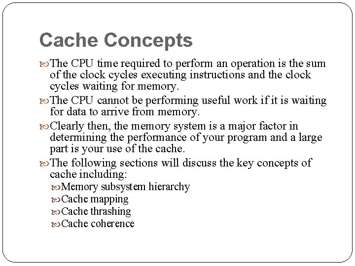
Cache Concepts The CPU time required to perform an operation is the sum of the clock cycles executing instructions and the clock cycles waiting for memory. The CPU cannot be performing useful work if it is waiting for data to arrive from memory. Clearly then, the memory system is a major factor in determining the performance of your program and a large part is your use of the cache. The following sections will discuss the key concepts of cache including: Memory subsystem hierarchy Cache mapping Cache thrashing Cache coherence

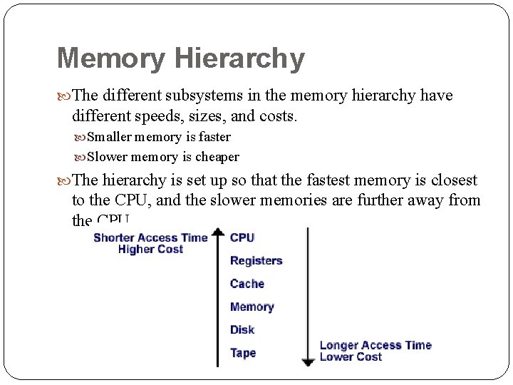
Memory Hierarchy The different subsystems in the memory hierarchy have different speeds, sizes, and costs. Smaller memory is faster Slower memory is cheaper The hierarchy is set up so that the fastest memory is closest to the CPU, and the slower memories are further away from the CPU.

Memory Hierarchy It's a hierarchy because every level is a subset of a level further away. All data in one level is found in the level below. The purpose of cache is to improve the memory access time to the processor. There is an overhead associated with it, but the benefits outweigh the cost. Registers are the sources and destinations of CPU data operations. They hold one data element each and are 32 bits or 64 bits wide. They are on-chip and built from SRAM. Computers usually have 32 or 64 registers. The Origin MIPS R 10000 has 64 physical 64 -bit registers of which 32 are available for floating-point operations.

Memory Hierarchy Main Memory Improvements A hardware improvement called interleaving reduces main memory access time. In interleaving, memory is divided into partitions or segments called memory banks. Consecutive data elements are spread across the banks. Each bank supplies one data element per bank cycle. Multiple data elements are read in parallel, one from each bank. The problem with interleaving is that the memory interleaving improvement assumes that memory is accessed sequentially. If there is 2 -way memory interleaving, but the code accesses every other location, there is no benefit. The bank cycle time is 4 -8 times the CPU clock cycle time so the main memory can’t keep up with the fast CPU and keep it busy with data. Large main memory with a cycle time comparable to the processor is not affordable.

Memory Hierarchy Principle of Locality The way your program operates follows the Principle of Locality. Temporal Locality: When an item is referenced, it will be referenced again soon. Spatial Locality: When an item is referenced, items whose addresses are nearby will tend to be referenced soon. Cache Line The overhead of the cache can be reduced by fetching a chunk or block of data elements. When a main memory access is made, a cache line of data is brought into the cache instead of a single data element. A cache line is defined in terms of a number of bytes. For example, a cache line is typically 32 or 128 bytes. This takes advantage of spatial locality. The additional elements in the cache line will most likely be needed soon. The cache miss rate falls as the size of the cache line increases, but there is a point of negative returns on the cache line size. When the cache line size becomes too large, the transfer time increases.

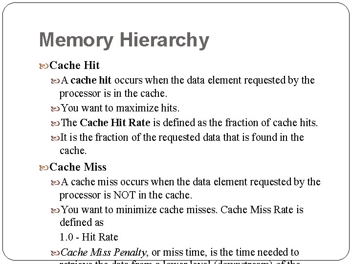
Memory Hierarchy Cache Hit A cache hit occurs when the data element requested by the processor is in the cache. You want to maximize hits. The Cache Hit Rate is defined as the fraction of cache hits. It is the fraction of the requested data that is found in the cache. Cache Miss A cache miss occurs when the data element requested by the processor is NOT in the cache. You want to minimize cache misses. Cache Miss Rate is defined as 1. 0 - Hit Rate Cache Miss Penalty, or miss time, is the time needed to

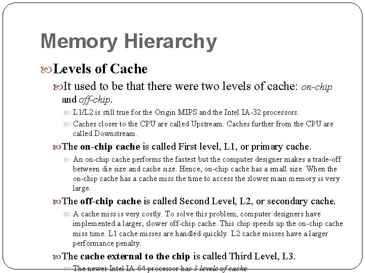
Memory Hierarchy Levels of Cache It used to be that there were two levels of cache: on-chip and off-chip. L 1/L 2 is still true for the Origin MIPS and the Intel IA-32 processors. Caches closer to the CPU are called Upstream. Caches further from the CPU are called Downstream. The on-chip cache is called First level, L 1, or primary cache. An on-chip cache performs the fastest but the computer designer makes a trade-off between die size and cache size. Hence, on-chip cache has a small size. When the on-chip cache has a cache miss the time to access the slower main memory is very large. The off-chip cache is called Second Level, L 2, or secondary cache. A cache miss is very costly. To solve this problem, computer designers have implemented a larger, slower off-chip cache. This chip speeds up the on-chip cache miss time. L 1 cache misses are handled quickly. L 2 cache misses have a larger performance penalty. The cache external to the chip is called Third Level, L 3. The newer Intel IA-64 processor has 3 levels of cache

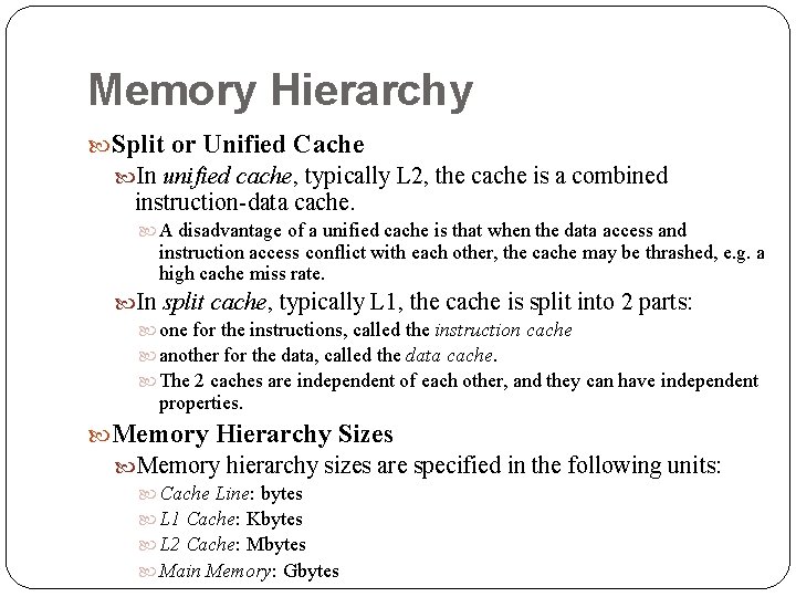
Memory Hierarchy Split or Unified Cache In unified cache, typically L 2, the cache is a combined instruction-data cache. A disadvantage of a unified cache is that when the data access and instruction access conflict with each other, the cache may be thrashed, e. g. a high cache miss rate. In split cache, typically L 1, the cache is split into 2 parts: one for the instructions, called the instruction cache another for the data, called the data cache. The 2 caches are independent of each other, and they can have independent properties. Memory Hierarchy Sizes Memory hierarchy sizes are specified in the following units: Cache Line: bytes L 1 Cache: Kbytes L 2 Cache: Mbytes Main Memory: Gbytes

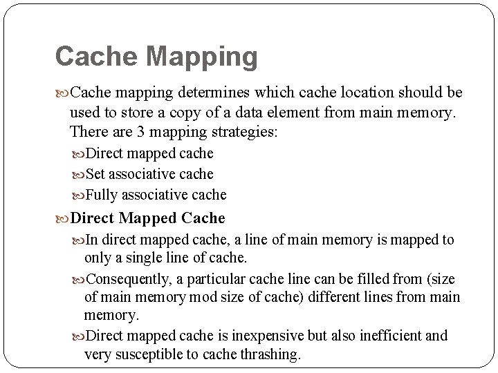
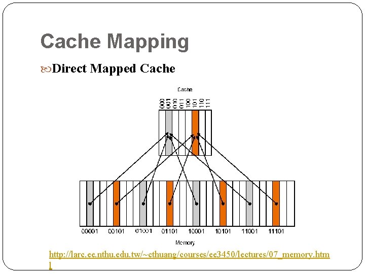
Cache Mapping Cache mapping determines which cache location should be used to store a copy of a data element from main memory. There are 3 mapping strategies: Direct mapped cache Set associative cache Fully associative cache Direct Mapped Cache In direct mapped cache, a line of main memory is mapped to only a single line of cache. Consequently, a particular cache line can be filled from (size of main memory mod size of cache) different lines from main memory. Direct mapped cache is inexpensive but also inefficient and very susceptible to cache thrashing.

Cache Mapping Direct Mapped Cache http: //larc. ee. nthu. edu. tw/~cthuang/courses/ee 3450/lectures/07_memory. htm l

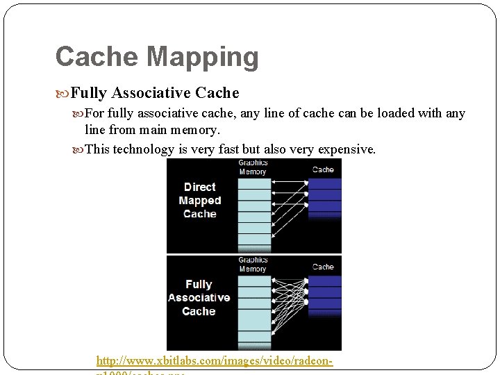
Cache Mapping Fully Associative Cache For fully associative cache, any line of cache can be loaded with any line from main memory. This technology is very fast but also very expensive. http: //www. xbitlabs. com/images/video/radeon-

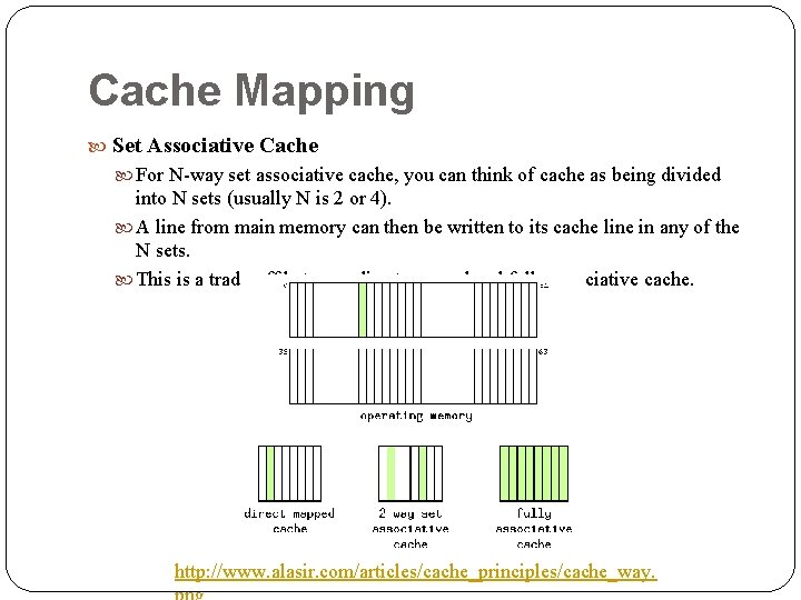
Cache Mapping Set Associative Cache For N-way set associative cache, you can think of cache as being divided into N sets (usually N is 2 or 4). A line from main memory can then be written to its cache line in any of the N sets. This is a trade-off between direct mapped and fully associative cache. http: //www. alasir. com/articles/cache_principles/cache_way.

Cache Mapping Cache Block Replacement With direct mapped cache, a cache line can only be mapped to one unique place in the cache. The new cache line replaces the cache block at that address. With set associative cache there is a choice of 3 strategies: 1. Random There is a uniform random replacement within the set of cache blocks. The advantage of random replacement is that it’s simple and inexpensive to implement. 2. LRU (Least Recently Used) The block that gets replaced is the one that hasn’t been used for the longest time. The principle of temporal locality tells us that recently used data blocks are likely to be used again soon. An advantage of LRU is that it preserves temporal locality. A disadvantage of LRU is that it’s expensive to keep track of cache access patterns. In empirical studies, there was little performance difference between LRU and Random. 3. FIFO (First In First Out) Replace the block that was brought in N accesses ago, regardless of the

Cache Thrashing Cache thrashing is a problem that happens when a frequently used cache line gets displaced by another frequently used cache line. Cache thrashing can happen for both instruction and data caches. The CPU can’t find the data element it wants in the cache and must make another main memory cache line access. The same data elements are repeatedly fetched into and displaced from the cache. Cache thrashing happens because the computational code statements have too many variables and arrays for the needed data elements to fit in cache. Cache lines are discarded and later retrieved. The arrays are dimensioned too large to fit in cache. The

Cache Coherence Cache coherence is maintained by an agreement between data stored in cache, other caches, and main memory. When the same data is being manipulated by different processors, they must inform each other of their modification of data. The term Protocol is used to describe how caches and main memory communicate with each other. It is the means by which all the memory subsystems maintain data coherence.

Cache Coherence Snoop Protocol All processors monitor the bus traffic to determine cache line status. Directory Based Protocol Cache lines contain extra bits that indicate which other processor has a copy of that cache line, and the status of the cache line – clean (cache line does not need to be sent back to main memory) or dirty (cache line needs to update main memory with content of cache line). Hardware Cache Coherence Cache coherence on the Origin computer is maintained in the hardware, transparent to the programmer.

Cache Coherence False sharing happens in a multiprocessor system as a result of maintaining cache coherence. Both processor A and processor B have the same cache line. A modifies the first word of the cache line. B wants to modify the eighth word of the cache line. But A has sent a signal to B that B’s cache line is invalid. B must fetch the cache line again before writing to it.

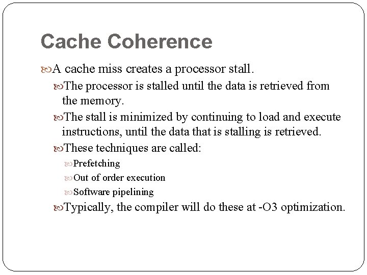
Cache Coherence A cache miss creates a processor stall. The processor is stalled until the data is retrieved from the memory. The stall is minimized by continuing to load and execute instructions, until the data that is stalling is retrieved. These techniques are called: Prefetching Out of order execution Software pipelining Typically, the compiler will do these at -O 3 optimization.

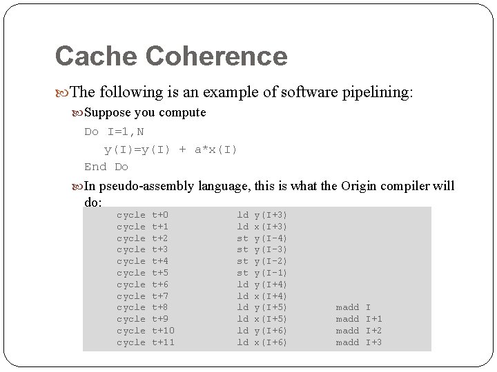
Cache Coherence The following is an example of software pipelining: Suppose you compute Do I=1, N y(I)=y(I) + a*x(I) End Do In pseudo-assembly language, this is what the Origin compiler will do: cycle cycle cycle t+0 t+1 t+2 t+3 t+4 t+5 t+6 t+7 t+8 t+9 t+10 t+11 ld ld st st ld ld ld y(I+3) x(I+3) y(I-4) y(I-3) y(I-2) y(I-1) y(I+4) x(I+4) y(I+5) x(I+5) y(I+6) x(I+6) madd I I+1 I+2 I+3

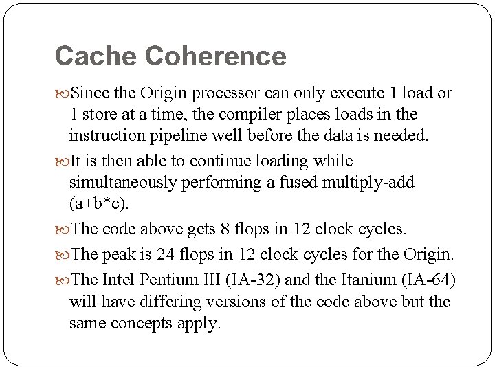
Cache Coherence Since the Origin processor can only execute 1 load or 1 store at a time, the compiler places loads in the instruction pipeline well before the data is needed. It is then able to continue loading while simultaneously performing a fused multiply-add (a+b*c). The code above gets 8 flops in 12 clock cycles. The peak is 24 flops in 12 clock cycles for the Origin. The Intel Pentium III (IA-32) and the Itanium (IA-64) will have differing versions of the code above but the same concepts apply.

Agenda 7 Cache Tuning 7. 1 Cache Concepts 7. 2 Cache Specifics 7. 2. 1 Cache on the SGI Origin 2000 7. 2. 2 Cache on the Intel Pentium III 7. 2. 3 Cache on the Intel Itanium 7. 2. 4 Cache Summary 7. 3 Code 0 ptimization 7. 4 Measuring Cache Performance 7. 5 Locating the Cache Problem 7. 6 Cache Tuning Strategy 7. 7 Preserve Spatial Locality 7. 8 Locality Problem 7. 9 Grouping Data Together 7. 10 Cache Thrashing Example 7. 11 Not Enough Cache 7. 12 Loop Blocking 7. 13 Further Information

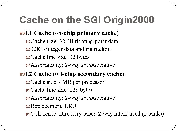
Cache on the SGI Origin 2000 L 1 Cache (on-chip primary cache) Cache size: 32 KB floating point data 32 KB integer data and instruction Cache line size: 32 bytes Associativity: 2 -way set associative L 2 Cache (off-chip secondary cache) Cache size: 4 MB per processor Cache line size: 128 bytes Associativity: 2 -way set associative Replacement: LRU Coherence: Directory based 2 -way interleaved (2 banks)

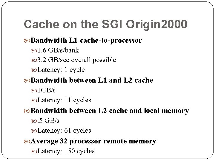
Cache on the SGI Origin 2000 Bandwidth L 1 cache-to-processor 1. 6 GB/s/bank 3. 2 GB/sec overall possible Latency: 1 cycle Bandwidth between L 1 and L 2 cache 1 GB/s Latency: 11 cycles Bandwidth between L 2 cache and local memory . 5 GB/s Latency: 61 cycles Average 32 processor remote memory Latency: 150 cycles

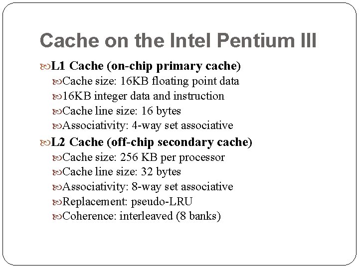
Cache on the Intel Pentium III L 1 Cache (on-chip primary cache) Cache size: 16 KB floating point data 16 KB integer data and instruction Cache line size: 16 bytes Associativity: 4 -way set associative L 2 Cache (off-chip secondary cache) Cache size: 256 KB per processor Cache line size: 32 bytes Associativity: 8 -way set associative Replacement: pseudo-LRU Coherence: interleaved (8 banks)

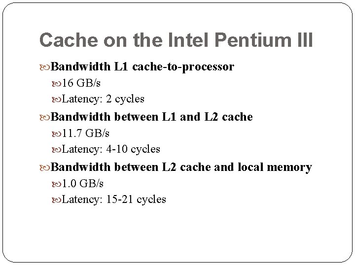
Cache on the Intel Pentium III Bandwidth L 1 cache-to-processor 16 GB/s Latency: 2 cycles Bandwidth between L 1 and L 2 cache 11. 7 GB/s Latency: 4 -10 cycles Bandwidth between L 2 cache and local memory 1. 0 GB/s Latency: 15 -21 cycles

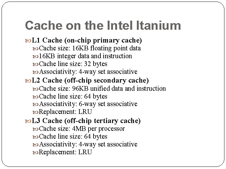
Cache on the Intel Itanium L 1 Cache (on-chip primary cache) Cache size: 16 KB floating point data 16 KB integer data and instruction Cache line size: 32 bytes Associativity: 4 -way set associative L 2 Cache (off-chip secondary cache) Cache size: 96 KB unified data and instruction Cache line size: 64 bytes Associativity: 6 -way set associative Replacement: LRU L 3 Cache (off-chip tertiary cache) Cache size: 4 MB per processor Cache line size: 64 bytes Associativity: 4 -way set associative Replacement: LRU

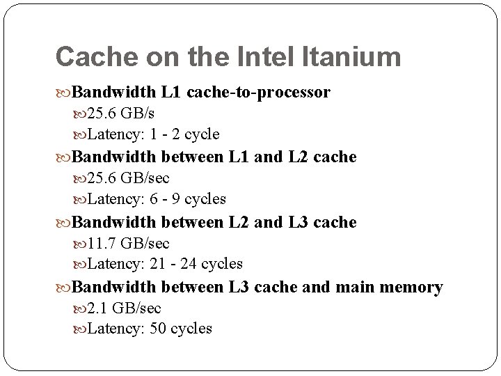
Cache on the Intel Itanium Bandwidth L 1 cache-to-processor 25. 6 GB/s Latency: 1 - 2 cycle Bandwidth between L 1 and L 2 cache 25. 6 GB/sec Latency: 6 - 9 cycles Bandwidth between L 2 and L 3 cache 11. 7 GB/sec Latency: 21 - 24 cycles Bandwidth between L 3 cache and main memory 2. 1 GB/sec Latency: 50 cycles

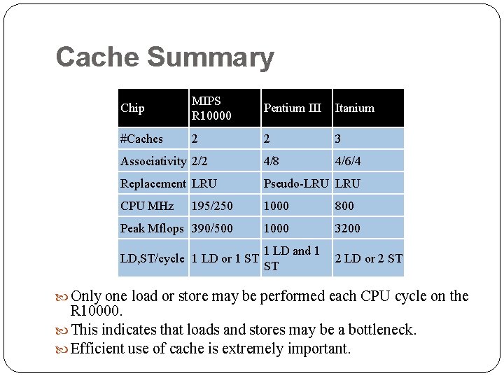
Cache Summary Chip MIPS R 10000 Pentium III Itanium #Caches 2 2 3 Associativity 2/2 4/8 4/6/4 Replacement LRU Pseudo-LRU CPU MHz 195/250 1000 800 Peak Mflops 390/500 1000 3200 LD, ST/cycle 1 LD or 1 ST 1 LD and 1 ST 2 LD or 2 ST Only one load or store may be performed each CPU cycle on the R 10000. This indicates that loads and stores may be a bottleneck. Efficient use of cache is extremely important.

Agenda 7 Cache Tuning 7. 1 Cache Concepts 7. 2 Cache Specifics 7. 3 Code 0 ptimization 7. 4 Measuring Cache Performance 7. 4. 1 Measuring Cache Performance on the SGI Origin 2000 7. 4. 2 Measuring Cache Performance on the Linux Clusters 7. 5 Locating the Cache Problem 7. 6 Cache Tuning Strategy 7. 7 Preserve Spatial Locality 7. 8 Locality Problem 7. 9 Grouping Data Together 7. 10 Cache Thrashing Example 7. 11 Not Enough Cache 7. 12 Loop Blocking 7. 13 Further Information

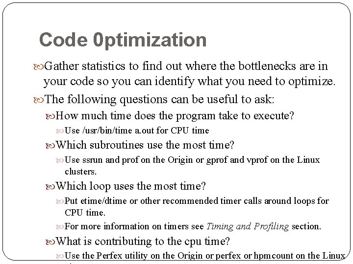
Code 0 ptimization Gather statistics to find out where the bottlenecks are in your code so you can identify what you need to optimize. The following questions can be useful to ask: How much time does the program take to execute? Use /usr/bin/time a. out for CPU time Which subroutines use the most time? Use ssrun and prof on the Origin or gprof and vprof on the Linux clusters. Which loop uses the most time? Put etime/dtime or other recommended timer calls around loops for CPU time. For more information on timers see Timing and Profiling section. What is contributing to the cpu time? Use the Perfex utility on the Origin or perfex or hpmcount on the Linux

Code 0 ptimization Some useful optimizing and profiling tools are etime/dtime/time perfex ssusage ssrun/prof gprof cvpav, cvd See the NCSA web pages on Compiler, Performance, and Productivity Tools http: //www. ncsa. uiuc. edu/User. Info/Resources/Software/Too ls/ for information on which tools are available on NCSA platforms.

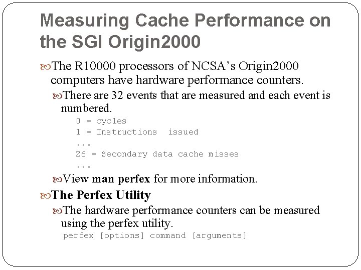
Measuring Cache Performance on the SGI Origin 2000 The R 10000 processors of NCSA’s Origin 2000 computers have hardware performance counters. There are 32 events that are measured and each event is numbered. 0 = cycles 1 = Instructions issued. . . 26 = Secondary data cache misses. . . View man perfex for more information. The Perfex Utility The hardware performance counters can be measured using the perfex utility. perfex [options] command [arguments]

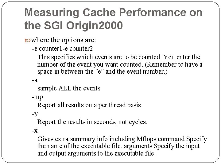
Measuring Cache Performance on the SGI Origin 2000 where the options are: -e counter 1 -e counter 2 This specifies which events are to be counted. You enter the number of the event you want counted. (Remember to have a space in between the "e" and the event number. ) -a sample ALL the events -mp Report all results on a per thread basis. -y Report the results in seconds, not cycles. -x Gives extra summary info including Mflops command Specify the name of the executable file. arguments Specify the input and output arguments to the executable file.

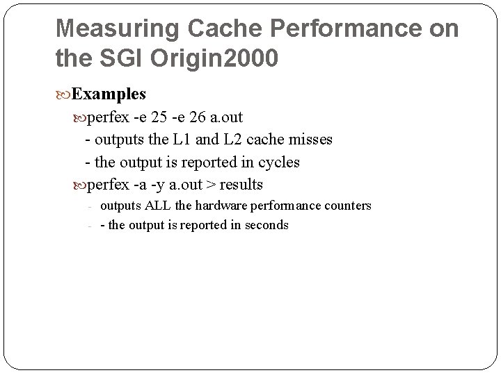
Measuring Cache Performance on the SGI Origin 2000 Examples perfex -e 25 -e 26 a. out - outputs the L 1 and L 2 cache misses - the output is reported in cycles perfex -a -y a. out > results - outputs ALL the hardware performance counters - - the output is reported in seconds

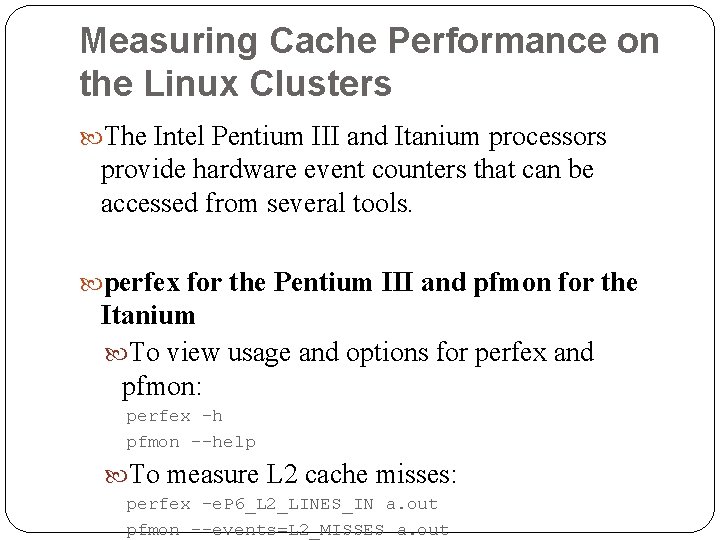
Measuring Cache Performance on the Linux Clusters The Intel Pentium III and Itanium processors provide hardware event counters that can be accessed from several tools. perfex for the Pentium III and pfmon for the Itanium To view usage and options for perfex and pfmon: perfex -h pfmon --help To measure L 2 cache misses: perfex –e. P 6_L 2_LINES_IN a. out pfmon –-events=L 2_MISSES a. out

Measuring Cache Performance on the Linux Clusters psrun [soft add +perfsuite] Another tool that provides access to the hardware event counter and also provides derived statistics is perfsuite. To add perfsuite's psrun to the current shell environment : soft add +perfsuite To measure cache misses: psrun a. out psprocess a. out*. xml

Agends 7 Cache Tuning 7. 1 Cache Concepts 7. 2 Cache Specifics 7. 3 Code 0 ptimization 7. 4 Measuring Cache Performance 7. 5 Locating the Cache Problem 7. 6 Cache Tuning Strategy 7. 7 Preserve Spatial Locality 7. 8 Locality Problem 7. 9 Grouping Data Together 7. 10 Cache Thrashing Example 7. 11 Not Enough Cache 7. 12 Loop Blocking 7. 13 Further Information

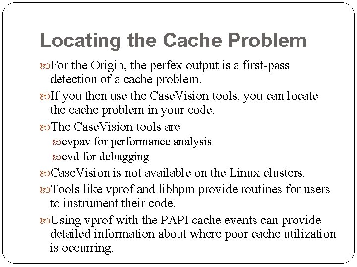
Locating the Cache Problem For the Origin, the perfex output is a first-pass detection of a cache problem. If you then use the Case. Vision tools, you can locate the cache problem in your code. The Case. Vision tools are cvpav for performance analysis cvd for debugging Case. Vision is not available on the Linux clusters. Tools like vprof and libhpm provide routines for users to instrument their code. Using vprof with the PAPI cache events can provide detailed information about where poor cache utilization is occurring.

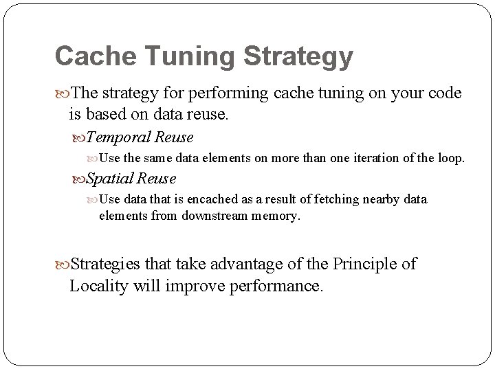
Cache Tuning Strategy The strategy for performing cache tuning on your code is based on data reuse. Temporal Reuse Use the same data elements on more than one iteration of the loop. Spatial Reuse Use data that is encached as a result of fetching nearby data elements from downstream memory. Strategies that take advantage of the Principle of Locality will improve performance.

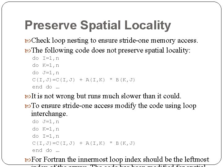
Preserve Spatial Locality Check loop nesting to ensure stride-one memory access. The following code does not preserve spatial locality: do I=1, n do K=1, n do J=1, n C(I, J)=C(I, J) + A(I, K) * B(K, J) end do … It is not wrong but runs much slower than it could. To ensure stride-one access modify the code using loop interchange. do J=1, n do K=1, n do I=1, n C(I, J)=C(I, J) + A(I, K) * B(K, J) end do … Fortran the innermost loop index should be the leftmost

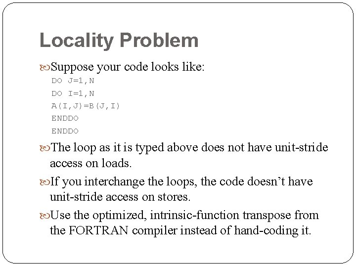
Locality Problem Suppose your code looks like: DO J=1, N DO I=1, N A(I, J)=B(J, I) ENDDO The loop as it is typed above does not have unit-stride access on loads. If you interchange the loops, the code doesn’t have unit-stride access on stores. Use the optimized, intrinsic-function transpose from the FORTRAN compiler instead of hand-coding it.

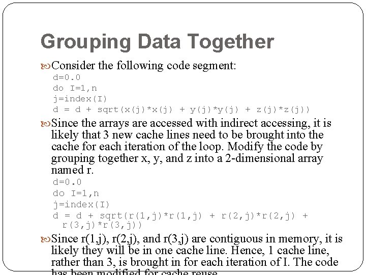
Grouping Data Together Consider the following code segment: d=0. 0 do I=1, n j=index(I) d = d + sqrt(x(j)*x(j) + y(j)*y(j) + z(j)*z(j)) Since the arrays are accessed with indirect accessing, it is likely that 3 new cache lines need to be brought into the cache for each iteration of the loop. Modify the code by grouping together x, y, and z into a 2 -dimensional array named r. d=0. 0 do I=1, n j=index(I) d = d + sqrt(r(1, j)*r(1, j) + r(2, j)*r(2, j) + r(3, j)*r(3, j)) Since r(1, j), r(2, j), and r(3, j) are contiguous in memory, it is likely they will be in one cache line. Hence, 1 cache line, rather than 3, is brought in for each iteration of I. The code

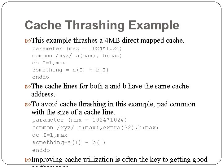
Cache Thrashing Example This example thrashes a 4 MB direct mapped cache. parameter (max = 1024*1024) common /xyz/ a(max), b(max) do I=1, max something = a(I) + b(I) enddo The cache lines for both a and b have the same cache address. To avoid cache thrashing in this example, pad common with the size of a cache line. parameter (max = 1024*1024) common /xyz/ a(max), extra(32), b(max) do I=1, max something=a(I) + b(I) enddo Improving cache utilization is often the key to getting good

Not Enough Cache Ideally you want the inner loop’s arrays and variables to fit into cache. If a scalar program won’t fit in cache, its parallel version may fit in cache with a large enough number of processors. This often results in super-linear speedup.

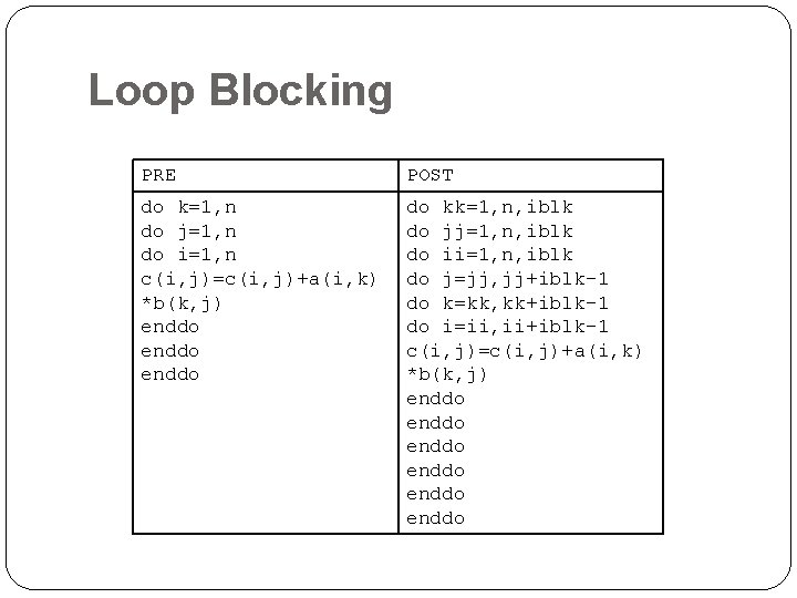
Loop Blocking This technique is useful when the arrays are too large to fit into the cache. Loop blocking uses strip mining of loops and loop interchange. A blocked loop accesses array elements in sections that optimally fit in the cache. It allows for spatial and temporal reuse of data, thus minimizing cache misses. The following example (next slide) illustrates loop blocking of matrix multiplication. The code in the PRE column depicts the original code, the POST column depicts the code when it is blocked.

Loop Blocking PRE POST do k=1, n do j=1, n do i=1, n c(i, j)=c(i, j)+a(i, k) *b(k, j) enddo do kk=1, n, iblk do jj=1, n, iblk do ii=1, n, iblk do j=jj, jj+iblk-1 do k=kk, kk+iblk-1 do i=ii, ii+iblk-1 c(i, j)=c(i, j)+a(i, k) *b(k, j) enddo enddo

Further Information Computer Organization and Design The Hardware/Software Interface, David A. Patterson and John L. Hennessy, Morgan Kaufmann Publishers, Inc. Computer Architecture A Quantitative Approach, John L. Hennessy and David A. Patterson, Morgan Kaufmann Publishers, Inc. The Cache Memory Book, Jim Handy, Academic Press High Performance Computing, Charles Severance, O’Reilly and Associates, Inc. A Practitioner’s Guide to RISC Microprocessor Architecture, Patrick H. Stakem, John Wiley & Sons, Inc. Tutorial on Optimization of Fortran, John Levesque, Applied Parallel Research Intel® Architecture Optimization Reference Manual Intel® Itanium® Processor Manuals