Parallel Computing CS 14 403 Basic Communication Operations

Parallel Computing CS 14. 403 Basic Communication Operations By Niranjan Lal CSE, MUST

Topic Overview • • One-to-All Broadcast and All-to-One Reduction All-to-All Broadcast and Reduction All-Reduce and Prefix-Sum Operations Scatter and Gather All-to-All Personalized Communication Circular Shift Improving the Speed of Some Communication Operations

Basic Communication Operations: Introduction • Many interactions in practical parallel programs occur in well-defined patterns involving groups of processors. • Efficient implementations of these operations can improve performance, reduce development effort and cost, and improve software quality. • Efficient implementations must leverage underlying architecture. For this reason, we refer to specific architectures here. • We select a descriptive set of architectures to illustrate the process of algorithm design.

Basic Communication Operations: Introduction • Group communication operations are built using point-topoint messaging primitives. • In most parallel algorithms, processes need to exchange data with other processes. This exchange of data can significantly impact the efficiency of parallel programs by introducing interaction delays during their execution. • Recall from our discussion of architectures that communicating a message of size m-word message over an uncongested network takes ts +mtw time for a simple exchange of an m-word message between two processes running on different nodes of an interconnection network with cut-through routing.

Basic Communication Operations: Introduction • Here ts is the latency or the startup time for the data transfer and tw is the per-word transfer time, which is inversely proportional to the available bandwidth between the nodes. • We use this as the basis for our analyses. Where necessary, we take congestion into account explicitly by scaling the tw term. • We assume that the network is bidirectional and that communication is single-ported.

Basic Communication Operations: Introduction • In this unit , we present algorithms to implement some commonly used communication patterns on simple interconnection networks, such as the linear array, twodimensional mesh, and the hypercube. • For instance, although it is unlikely that large scale parallel computers will be based on the linear array or ring topology, it is important to understand various communication operations in the context of linear arrays because the rows and columns of meshes are linear arrays. .

Basic Communication Operations: Introduction – Parallel algorithms that perform row-wise or column-wise communication on meshes use linear array algorithms. – The algorithms for a number of communication operations on a mesh are simple extensions of the corresponding linear array algorithms to two dimensions. – Furthermore, parallel algorithms using regular data structures such as arrays often map naturally onto oneor two-dimensional arrays of processes. – The hypercube architecture, on the other hand, is interesting because many algorithms with recursive interaction patterns map naturally onto a hypercube topology.

Basic Communication Operations: Introduction • In the following sections we describe various communication operations and derive expressions for their time complexity. • We assume that the interconnection network supports cut-through routing discussed previously and that the communication time between any pair of nodes is practically independent of the number of intermediate nodes along the paths between them. • We also assume that the communication links are bidirectional; that is, two directly-connected nodes can send messages of size m to each other simultaneously in time ts + twm.

Basic Communication Operations: Introduction • We assume a single-port communication model, in which a node can send a message on only one of its links at a time. Similarly, it can receive a message on only one link at a time. • However, a node can receive a message while sending another message at the same time on the same or a different link.

Basic Communication Operations: Introduction • Many of the operations described here have duals and other related operations that we can perform by using procedures very similar to those for the original operations. • Many algorithms for all-to-one and all-to-all communication are simply reversals and duals of the one-to-all broadcast. • The dual of a communication operation is the opposite of the original operation and can be performed by reversing the direction and sequence of messages in the original operation. • We will mention such operations wherever applicable.

One-to-All Broadcast and All-to-One Reduction • Parallel algorithms often require a single process to send identical data to all other processes or to a subset of them. This operation is known as one-to-all broadcast. • Initially, only the source process has the data of size m that needs to be broadcast. At the termination of the procedure, there are p copies of the initial data – one belonging to each process. The dual of one-to-all broadcast is allto-one reduction.

One-to-All Broadcast and All-to-One Reduction • In an all-to-one reduction operation, each of the p participating processes starts with a buffer M containing m words. • The data from all processes are combined through an associative operator and accumulated at a single destination process into one buffer of size m. • Reduction can be used to find the sum, product, maximum, or minimum of sets of numbers – the ith word of the accumulated M is the sum, product, maximum, or minimum of the ith words of each of the original buffers. • Next Figure shows one to-all broadcast and all-to-one reduction among p processes.

One-to-All Broadcast and All-to-One Reduction One-to-all broadcast and all-to-one reduction among processors. One-to-all broadcast and all-to-one reduction are used in several important parallel algorithms including matrix-vector multiplication, Gaussian elimination, shortest paths, and vector inner product. In the following subsections, we consider the implementation of one-to-all broadcast in detail on a variety of interconnection topologies.

1. Ring or Linear Array • A naive way to perform one-to-all broadcast is to sequentially send p – 1 messages from the source to the other p - 1 processes. However, this is inefficient because the source process becomes a bottleneck. • Moreover, the communication network is underutilized because only the connection between a single pair of nodes is used at a time. A better broadcast algorithm can be devised using a technique commonly known as recursive doubling. • The source process first sends the message to another process. Now both these processes can simultaneously send the message to two other processes that are still waiting for the message. By continuing this procedure until all the processes have received the data, the message can be broadcast in log p steps.

One-to-All Broadcast One-to-all broadcast on an eight-node ring. Node 0 is the source of the broadcast. Each message transfer step is shown by a numbered, dotted arrow from the source of the message to its destination. The number on an arrow indicates the time step during which the message is transferred.

One-to-All Broadcast • Note that on a linear array, the destination node to which the message is sent in each step must be carefully chosen. • In Figure 4. 2 , the message is first sent to the farthest node (4) from the source (0). • In the second step, the distance between the sending and receiving nodes is halved, and so on. • The message recipients are selected in this manner at each step to avoid congestion on the network. • For example, if node 0 sent the message to node 1 in the first step and then nodes 0 and 1 attempted to send messages to nodes 2 and 3, respectively, in the second step, the link between nodes 1 and 2 would be congested as it would be a part of the shortest route for both the messages in the second step.

All-to-One Reduction • Reduction on a linear array can be performed by simply reversing the direction and the sequence of communication, as shown in Figure 4. 3. • In the first step, each odd numbered node sends its buffer to the even numbered node just before itself, where the contents of the two • buffers are combined into one. • After the first step, there are four buffers left to be reduced on nodes 0, 2, 4, and 6, respectively. In the second step, the contents of the buffers on nodes 0 and 2 are accumulated on node 0 and those on nodes 6 and 4 are accumulated on node 4. • Finally, node 4 sends its buffer to node 0, which computes the final result of the reduction.

All-to-One Reduction on an eight-node ring with node 0 as the destination of the reduction.

Broadcast and Reduction: Example Consider the problem of multiplying a matrix with a vector. • The n x n matrix is assigned to an n x n (virtual) processor grid. The vector is assumed to be on the first row of processors. • The first step of the product requires a one-to-all broadcast of the vector element along the corresponding column of processors. This can be done concurrently for all n columns. • The processors compute local product of the vector element and the local matrix entry. • In the final step, the results of these products are accumulated to the first row using n concurrent all-to-one reduction operations along the columns (using the sum operation).

Broadcast and Reduction: Matrix-Vector Multiplication Example One-to-all broadcast and all-to-one reduction in the multiplication of a 4 x 4 matrix with a 4 x 1 vector.

Broadcast and Reduction on a Mesh • We can view each row and column of a square mesh of p nodes as a linear array of √p nodes. • Broadcast and reduction operations can be performed in two steps - the first step does the operation along a row and the second step along each column concurrently. • This process generalizes to higher dimensions as well.

Broadcast and Reduction on a Mesh: Example One-to-all broadcast on a 16 -node mesh.

Broadcast and Reduction on a Hypercube • A hypercube with 2 d nodes can be regarded as a ddimensional mesh with two nodes in each dimension. • The mesh algorithm can be generalized to a hypercube and the operation is carried out in d (= log p) steps.

Broadcast and Reduction on a Hypercube: Example One-to-all broadcast on a three-dimensional hypercube. The binary representations of node labels are shown in parentheses.

Broadcast and Reduction on a Balanced Binary Tree • Consider a binary tree in which processors are (logically) at the leaves and internal nodes are routing nodes. • Assume that source processor is the root of this tree. In the first step, the source sends the data to the right child (assuming the source is also the left child). The problem has now been decomposed into two problems with half the number of processors.

Broadcast and Reduction on a Balanced Binary Tree One-to-all broadcast on an eight-node tree.

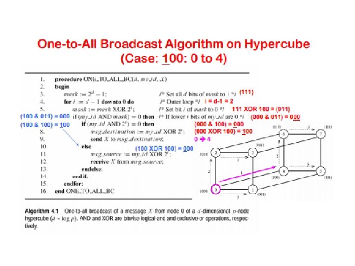
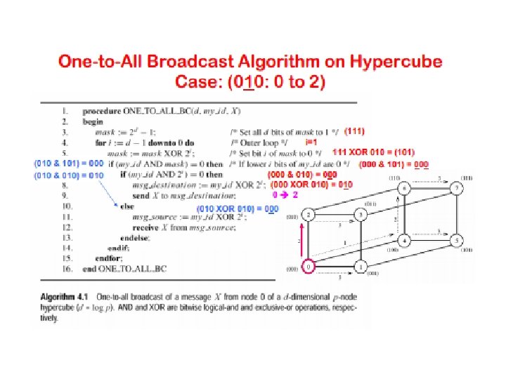
Broadcast and Reduction Algorithms • All of the algorithms described above are adaptations of the same algorithmic template. • We illustrate the algorithm for a hypercube, but the algorithm, as has been seen, can be adapted to other architectures. • The hypercube has 2 d nodes and my_id is the label for a node. • X is the message to be broadcast, which initially resides at the source node 0.

Broadcast and Reduction Algorithms One-to-all broadcast of a message X from source on a hypercube.

Broadcast and Reduction Algorithms Single-node accumulation on a d-dimensional hypercube. Each node contributes a message X containing m words, and node 0 is the destination.

Cost Analysis • The broadcast or reduction procedure involves log p point-to-point simple message transfers, each at a time cost of ts + twm. • The total time is therefore given by:

All-to-All Broadcast and Reduction • Generalization of broadcast in which each processor is the source as well as destination. • A process sends the same m-word message to every other process, but different processes may broadcast different messages. • All-to-all broadcast is used in matrix operations, including matrix multiplication and matrix-vector multiplication. The dual of all-to-all broadcast is all-to-all reduction, in which every node is the destination of an all-to-one reduction (Problem 4. 8). Next illustrates all-to-all broadcast and all-to-all reduction.

All-to-All Broadcast and Reduction All-to-all broadcast and all-to-all reduction.

All-to-All Broadcast and Reduction on a Ring • Simplest approach: perform p one-to-all broadcasts. This is not the most efficient way, though. • Each node first sends to one of its neighbors the data it needs to broadcast. • In subsequent steps, it forwards the data received from one of its neighbors to its other neighbor. • The algorithm terminates in p-1 steps. • The following sections describe all-to-all broadcast on linear array, mesh, and hypercube topologies.

All-to-All Broadcast and Reduction on a Ring • • • While performing all-to-all broadcast on a linear array or a ring, all communication links can be kept busy simultaneously until the operation is complete because each node always has some information that it can pass along to its neighbor. Each node first sends to one of its neighbors the data it needs to broadcast. In subsequent steps, it forwards the data received from one of its neighbors to its other neighbor. Figure 4. 9 illustrates all-to-all broadcast for an eight-node ring. The same procedure would also work on a linear array with bidirectional links. As with the previous figures, the integer label of an arrow indicates the time step during which the message is sent.

All-to-All Broadcast and Reduction on a Ring • • • Next Figure shows All-to-all broadcast on an eight-node ring. The label of each arrow shows the time step and, within parentheses, the label of the node that owned the current message being transferred before the beginning of the broadcast. The number(s) in parentheses next to each node are the labels of nodes from which data has been received prior to the current communication step. Only the first, second, and last communication steps are shown. In all-to-all broadcast, p different messages circulate in the p-node ensemble. In Figure 4. 9, each message is identified by its initial source, whose label appears in parentheses along with the time step. For instance, the arc labeled 2 (7) between nodes 0 and 1 represents the data communicated in time step 2 that node 0 received from node 7 in the preceding step. As Figure 4. 9 shows, if communication is performed circularly in a single direction, then each node receives all (p - 1) pieces of information from all other nodes in (p - 1) steps.

All-to-All Broadcast and Reduction on a Ring All-to-all broadcast on an eight-node ring.

All-to-All Broadcast and Reduction on a Ring All-to-all broadcast on a p-node ring.

All-to-all Broadcast on a Mesh • Performed in two phases - in the first phase, each row of the mesh performs an all-to-all broadcast using the procedure for the linear array. • In this phase, all nodes collect √p messages p=8, √p=2. 8=3 corresponding to the √p nodes of their respective rows. Each node consolidates this information into a single message of size m√p. • The second communication phase is a column wise all-to -all broadcast of the consolidated messages.

All-to-all Broadcast on a Mesh All-to-all broadcast on a 3 x 3 mesh. The groups of nodes communicating with each other in each phase are enclosed by dotted boundaries. By the end of the second phase, all nodes get (0, 1, 2, 3, 4, 5, 6, 7) (that is, a message from each node).

All-to-all Broadcast on a Mesh All-to-all broadcast on a square mesh of p nodes.

All-to-all broadcast on a Hypercube • Generalization of the mesh algorithm to log p dimensions. • Message size doubles at each of the log p steps.

All-to-all broadcast on a Hypercube All-to-all broadcast on an eight-node hypercube.

All-to-all broadcast on a Hypercube All-to-all broadcast on a d-dimensional hypercube.

All-to-all Reduction • Similar communication pattern to all-to-all broadcast, except in the reverse order. • On receiving a message, a node must combine it with the local copy of the message that has the same destination as the received message before forwarding the combined message to the next neighbor.

Cost Analysis • On a ring, the time is given by: (ts + twm)(p-1). • On a mesh, the time is given by: 2 ts(√p – 1) + twm(p-1). • On a hypercube, we have:

All-to-all broadcast: Notes • All of the algorithms presented above are asymptotically optimal in message size. • It is not possible to port algorithms for higher dimensional networks (such as a hypercube) into a ring because this would cause contention.

All-to-all broadcast: Notes Contention for a channel when the hypercube is mapped onto a ring.

All-Reduce and Prefix-Sum Operations • In all-reduce, each node starts with a buffer of size m and the final results of the operation are identical buffers of size m on each node that are formed by combining the original p buffers using an associative operator. • Identical to all-to-one reduction followed by a one-to-all broadcast. This formulation is not the most efficient. Uses the pattern of all-to-all broadcast, instead. The only difference is that message size does not increase here. Time for this operation is (ts + twm) log p. • Different from all-to-all reduction, in which p simultaneous all-to-one reductions take place, each with a different destination for the result.

The Prefix-Sum Operation • Given p numbers n 0, n 1, …, np-1 (one on each node), the problem is to compute the sums sk = ∑ik= 0 ni for all k between 0 and p-1. • Initially, nk resides on the node labeled k, and at the end of the procedure, the same node holds Sk.

The Prefix-Sum Operation • Figure 4. 13(Figure in Next Slide) illustrates the prefix sums procedure for an eight-node hypercube. This figure is a modification of Figure 4. 11(All-to-all broadcast on an eightnode hypercube). • The modification is required to accommodate the fact that in prefix sums the node with label k uses information from only the k-node subset of those nodes whose labels are less than or equal to k. • To accumulate the correct prefix sum, every node maintains an additional result buffer. This buffer is denoted by square brackets in Figure 4. 13. • At the end of a communication step, the content of an incoming message is added to the result buffer only if the message comes from a node with a smaller label than that of the recipient node.

The Prefix-Sum Operation • The contents of the outgoing message (denoted by parentheses in the figure) are updated with every incoming message, just as in the case of the all-reduce operation. • For instance, after the first communication step, nodes 0, 2, and 4 do not add the data received from nodes 1, 3, and 5 to their result buffers. However, the contents of the outgoing messages for the next step are updated.

The Prefix-Sum Operation Computing prefix sums on an eight-node hypercube. At each node, square brackets show the local prefix sum accumulated in the result buffer and parentheses enclose the contents of the outgoing message buffer for the next step.

The Prefix-Sum Operation • The operation can be implemented using the all-to-all broadcast kernel. • We must account for the fact that in prefix sums the node with label k uses information from only the k-node subset whose labels are less than or equal to k. • This is implemented using an additional result buffer. The content of an incoming message is added to the result buffer only if the message comes from a node with a smaller label than the recipient node. • The contents of the outgoing message (denoted by parentheses in the figure) are updated with every incoming message.

The Prefix-Sum Operation Prefix sums on a d-dimensional hypercube.

Scatter and Gather • In the scatter operation, a single node sends a unique message of size m to every other node (also called a one -to-all personalized communication). • In the gather operation, a single node collects a unique message from each node. • While the scatter operation is fundamentally different from broadcast, the algorithmic structure is similar, except for differences in message sizes (messages get smaller in scatter and stay constant in broadcast). • The gather operation is exactly the inverse of the scatter operation and can be executed as such.

Gather and Scatter Operations Scatter and gather operations.

Example of the Scatter Operation The scatter operation on an eight-node hypercube.

Cost of Scatter and Gather • There are log p steps, in each step, the machine size halves and the data size halves. • We have the time for this operation to be: • This time holds for a linear array as well as a 2 -D mesh. • These times are asymptotically optimal in message size.

All-to-All Personalized Communication • Each node has a distinct message of size m for every other node. • This is unlike all-to-all broadcast, in which each node sends the same message to all other nodes. • All-to-all personalized communication is also known as total exchange.

All-to-All Personalized Communication All-to-all personalized communication.

All-to-All Personalized Communication: Example • Consider the problem of transposing a matrix. • Each processor contains one full row of the matrix. • The transpose operation in this case is identical to an allto-all personalized communication operation.

All-to-All Personalized Communication: Example All-to-all personalized communication in transposing a 4 x 4 matrix using four processes.

All-to-All Personalized Communication on a Ring, Hypercube • Each node sends all pieces of data as one consolidated message of size m(p – 1) to one of its neighbors. • Each node extracts the information meant for it from the data received, and forwards the remaining (p – 2) pieces of size m each to the next node. • The algorithm terminates in p – 1 steps. • The size of the message reduces by m at each step.

All-to-All Personalized Communication on a Ring All-to-all personalized communication on a six-node ring. The label of each message is of the form {x, y}, where x is the label of the node that originally owned the message, and y is the label of the node that is the final destination of the message. The label ({x 1, y 1}, {x 2, y 2}, …, {xn, yn}, indicates a message that is formed by concatenating n individual messages.

All-to-All Personalized Communication on a Ring: Cost • We have p – 1 steps in all. • In step i, the message size is m(p – i). • The total time is given by: • The tw term in this equation can be reduced by a factor of 2 by communicating messages in both directions.

All-to-All Personalized Communication on a Mesh • Each node first groups its p messages according to the columns of their destination nodes. • All-to-all personalized communication is performed independently in each row with clustered messages of size m√p. • Messages in each node are sorted again, this time according to the rows of their destination nodes. • All-to-all personalized communication is performed independently in each column with clustered messages of size m√p.

All-to-All Personalized Communication on a Mesh The distribution of messages at the beginning of each phase of all-to-all personalized communication on a 3 x 3 mesh. At the end of the second phase, node i has messages ({0, i}, …, {8, i}), where 0 ≤ i ≤ 8. The groups of nodes communicating together in each phase are enclosed in dotted boundaries.

All-to-All Personalized Communication on a Mesh: Cost • Time for the first phase is identical to that in a ring with √p processors, i. e. , (ts + twmp/2)(√p – 1). • Time in the second phase is identical to the first phase. Therefore, total time is twice of this time, i. e. , • It can be shown that the time for rearrangement is less much less than this communication time.

All-to-All Personalized Communication on a Hypercube • Generalize the mesh algorithm to log p steps. • At any stage in all-to-all personalized communication, every node holds p packets of size m each. • While communicating in a particular dimension, every node sends p/2 of these packets (consolidated as one message). • A node must rearrange its messages locally before each of the log p communication steps.

All-to-All Personalized Communication on a Hypercube An all-to-all personalized communication algorithm on a three-dimensional hypercube.

All-to-All Personalized Communication on a Hypercube: Cost • We have log p iterations and mp/2 words are communicated in each iteration. Therefore, the cost is: • This is not optimal!

All-to-All Personalized Communication on a Hypercube: Optimal Algorithm • Each node simply performs p – 1 communication steps, exchanging m words of data with a different node in every step. • A node must choose its communication partner in each step so that the hypercube links do not suffer congestion. • In the jth communication step, node i exchanges data with node (i XOR j). • In this schedule, all paths in every communication step are congestion-free, and none of the bidirectional links carry more than one message in the same direction.

All-to-All Personalized Communication on a Hypercube: Optimal Algorithm Seven steps in all-to-all personalized communication on an eight-node hypercube.

All-to-All Personalized Communication on a Hypercube: Optimal Algorithm A procedure to perform all-to-all personalized communication on a ddimensional hypercube. The message Mi, j initially resides on node i and is destined for node j.

All-to-All Personalized Communication on a Hypercube: Cost Analysis of Optimal Algorithm • There are p – 1 steps and each step involves noncongesting message transfer of m words. • We have: • This is asymptotically optimal in message size.

Circular Shift • A special permutation in which node i sends a data packet to node (i + q) mod p in a p-node ensemble (0 ≤ q ≤ p).

Circular Shift • A special permutation in which node i sends a data packet to node (i + q) mod p in a p-node ensemble (0 ≤ q ≤ p). 1. 2.

Circular Shift on a Mesh • The implementation on a ring is rather intuitive. It can be performed in min{q, p – q} neighbor communications. • Mesh algorithms follow from this as well. We shift in one direction (all processors) followed by the next direction. • The associated time has an upper bound of:

Circular Shift on a Mesh The communication steps in a circular 5 -shift on a 4 x 4 mesh.

Circular Shift on a Hypercube • Map a linear array with 2 d nodes onto a d-dimensional hypercube. • To perform a q-shift, we expand q as a sum of distinct powers of 2. • If q is the sum of s distinct powers of 2, then the circular q-shift on a hypercube is performed in s phases. • The time for this is upper bounded by: • If E-cube routing is used, this time can be reduced to

Circular Shift on a Hypercube The mapping of an eight-node linear array onto a three-dimensional hypercube to perform a circular 5 -shift as a combination of a 4 -shift and a 1 -shift.

Circular Shift on a Hypercube Circular q-shifts on an 8 -node hypercube for 1 ≤ q < 8.

Improving Performance of Operations • Splitting and routing messages into parts: If the message can be split into p parts, a one-to-all broadcast can be implemented as a scatter operation followed by an all-toall broadcast operation. The time for this is: • All-to-one reduction can be performed by performing allto-all reduction (dual of all-to-all broadcast) followed by a gather operation (dual of scatter).

Improving Performance of Operations • Since an all-reduce operation is semantically equivalent to an all-to-one reduction followed by a one-to-all broadcast, the asymptotically optimal algorithms for these two operations can be used to construct a similar algorithm for the all-reduce operation. • The intervening gather and scatter operations cancel each other. Therefore, an all-reduce operation requires an all-to-all reduction and an all-to-all broadcast.