Parallel Computing 6 Performance Analysis Ondej Jakl Institute

Parallel Computing 6 Performance Analysis Ondřej Jakl Institute of Geonics, Academy of Sci. of the 1 CR

Outline of the lecture • • Performance models Execution time: computation, communication, idle Experimental studies Speed, efficiency, cost Amdahl’s and Gustafson’s law Scalability – fixed and scaled problem size Isoefficiency function 2

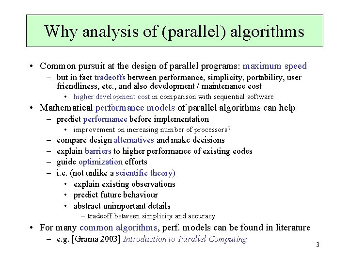
Why analysis of (parallel) algorithms • Common pursuit at the design of parallel programs: maximum speed – but in fact tradeoffs between performance, simplicity, portability, user friendliness, etc. , and also development / maintenance cost • higher development cost in comparison with sequential software • Mathematical performance models of parallel algorithms can help – predict performance before implementation • improvement on increasing number of processors? – – compare design alternatives and make decisions explain barriers to higher performance of existing codes guide optimization efforts i. e. (not unlike a scientific theory) • explain existing observations • predict future behaviour • abstract unimportant details – tradeoff between simplicity and accuracy • For many common algorithms, perf. models can be found in literature – e. g. [Grama 2003] Introduction to Parallel Computing 3

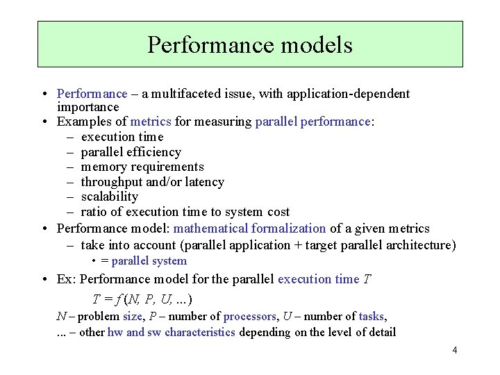
Performance models • Performance – a multifaceted issue, with application-dependent importance • Examples of metrics for measuring parallel performance: – execution time – parallel efficiency – memory requirements – throughput and/or latency – scalability – ratio of execution time to system cost • Performance model: mathematical formalization of a given metrics – take into account (parallel application + target parallel architecture) • = parallel system • Ex: Performance model for the parallel execution time T T = f (N, P, U, . . . ) N – problem size, P – number of processors, U – number of tasks, . . . – other hw and sw characteristics depending on the level of detail 4

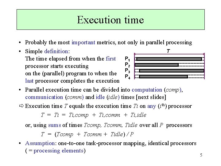
Execution time • Probably the most important metrics, not only in parallel processing T • Simple definition: The time elapsed from when the first P 1 P 2 processor starts executing P on the (parallel) program to when the P 3 4 last processor completes the execution • Parallel execution time can be divided into computation (comp), communication (comm) and idle (idle) times [next slides] Execution time T equals the execution time Ti on any (ith) processor T = Ti, comp + Ti, comm + Ti, idle or, using sums of times Tcomp, Tcomm, Tidle over all P processors T = (Tcomp + Tcomm + Tidle) / P • Assumption: one-to-one task-processor mapping, identical processors ( = processing elements) 5

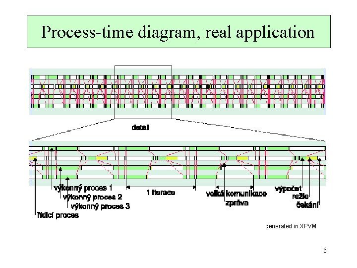
Process-time diagram, real application generated in XPVM 6

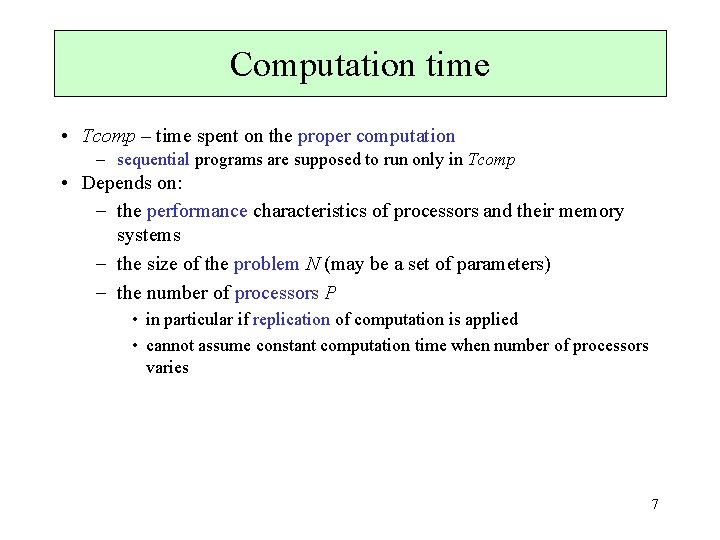
Computation time • Tcomp – time spent on the proper computation – sequential programs are supposed to run only in Tcomp • Depends on: the performance characteristics of processors and their memory systems the size of the problem N (may be a set of parameters) the number of processors P • in particular if replication of computation is applied • cannot assume constant computation time when number of processors varies 7

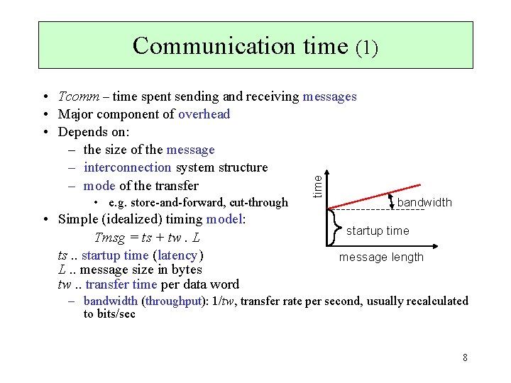
Communication time (1) • e. g. store-and-forward, cut-through • Simple (idealized) timing model: Tmsg = ts + tw. L ts. . startup time (latency) L. . message size in bytes tw. . transfer time per data word time • Tcomm – time spent sending and receiving messages • Major component of overhead • Depends on: – the size of the message – interconnection system structure – mode of the transfer bandwidth startup time message length bandwidth (throughput): 1/tw, transfer rate per second, usually recalculated to bits/sec 8

Communication time (2) • Substantial platform-dependent differences in ts, tw – cf. [Foster 1995] – measurements necessary (ping-pong test) – great impact on the parallelization approach • Ex. IBM SP timings: to : tw : ts = 1 : 55 : 8333 • to. . arithmetic operation time – latency dominates with small messages! • Internode versus intranode communication: • location of the communicating tasks: the same x different computing nodes – intranode communication in general conceived faster • valid e. g. on Ethernet networks • on supercomputers often quite comparable 9

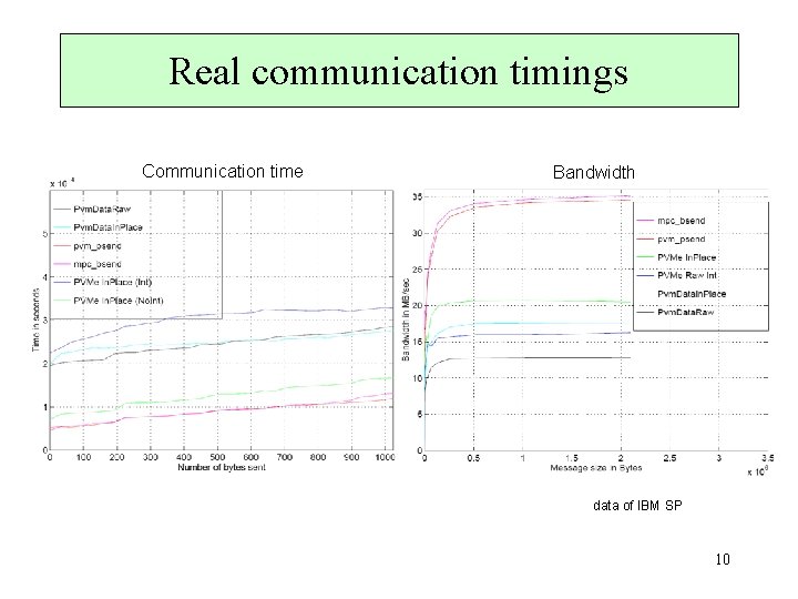
Real communication timings Communication time Bandwidth data of IBM SP 10

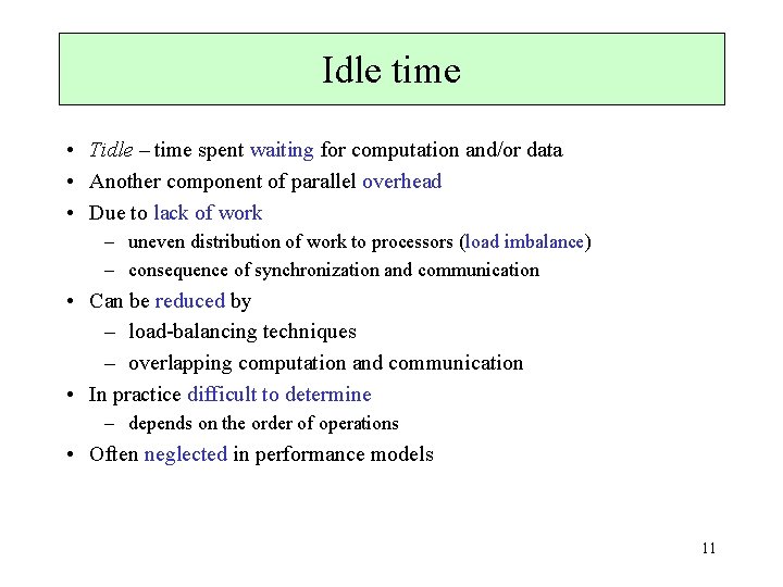
Idle time • Tidle – time spent waiting for computation and/or data • Another component of parallel overhead • Due to lack of work – uneven distribution of work to processors (load imbalance) – consequence of synchronization and communication • Can be reduced by – load-balancing techniques – overlapping computation and communication • In practice difficult to determine – depends on the order of operations • Often neglected in performance models 11

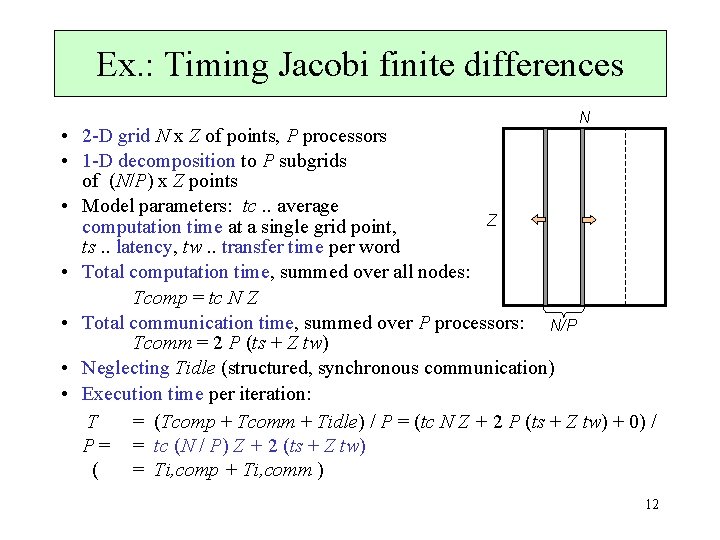
Ex. : Timing Jacobi finite differences N • 2 -D grid N x Z of points, P processors • 1 -D decomposition to P subgrids of (N/P) x Z points • Model parameters: tc. . average Z computation time at a single grid point, ts. . latency, tw. . transfer time per word • Total computation time, summed over all nodes: Tcomp = tc N Z • Total communication time, summed over P processors: N/P Tcomm = 2 P (ts + Z tw) • Neglecting Tidle (structured, synchronous communication) • Execution time per iteration: T = (Tcomp + Tcomm + Tidle) / P = (tc N Z + 2 P (ts + Z tw) + 0) / P = = tc (N / P) Z + 2 (ts + Z tw) ( = Ti, comp + Ti, comm ) 12

Reducing model complexity • Idealized multicomputer – no low-level hardware details, e. g. memory hierarchies, network topologies • Scale analysis – e. g. neglect one-time initialization step of an iterative algorithm • Empirical constants for model calibration • instead of modelling details • Trade-off between model complexity and acceptable accuracy 13

Experimental studies • Parallel computing is primarily an experimental discipline • Goals of experimental studies: – parameters for performance models (e. g. ts, tw in Tcomm) – comparison of observed and modelled performance – calibration of performance models • Design of experiments – issues: – data to be measured – measurement methods and tools – accuracy and reproducibility (always repeat to verify!) • Often greater variations in results – possible causes: – – – a nondeterministic algorithm (e. g. due to random numbers) timer problems (inaccurate, limited resolution) startup and shutdown costs (expensive, system dependent) interference from other programs (even on dedicated processors) communication contention (e. g. on the Ethernet) random resource allocation (if processor nodes are not equivalent) 14

Comparative performance metrics • Execution time not always convenient – varies with problem size – comparison with original sequential code needed • More adequate measures of parallelization quality: – speedup – efficiency – cost • Base for qualitative analysis 15

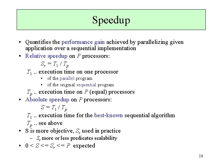
Speedup • Quantifies the performance gain achieved by parallelizing given application over a sequential implementation • Relative speedup on P processors: Sr = T 1 / Tp T 1. . execution time on one processor • of the parallel program • of the original sequential program Tp. . execution time on P (equal) processors • Absolute speedup on P processors: S = T 1 / Tp T 1. . execution time for the best-known sequential algorithm Tp. . see above • S is more objective, Sr used in practice – Sr more or less predicates scalability • 0 < S <= Sr <= P expected 16

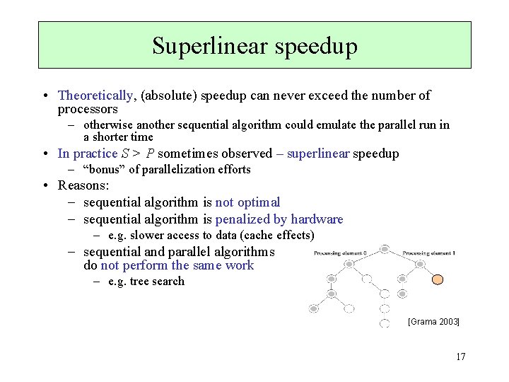
Superlinear speedup • Theoretically, (absolute) speedup can never exceed the number of processors – otherwise another sequential algorithm could emulate the parallel run in a shorter time • In practice S > P sometimes observed – superlinear speedup – “bonus” of parallelization efforts • Reasons: sequential algorithm is not optimal sequential algorithm is penalized by hardware e. g. slower access to data (cache effects) sequential and parallel algorithms do not perform the same work e. g. tree search [Grama 2003] 17

Typical speedup curves linear speedup Program 1 superlinear speedup Program 2 [Lin 2009] 18

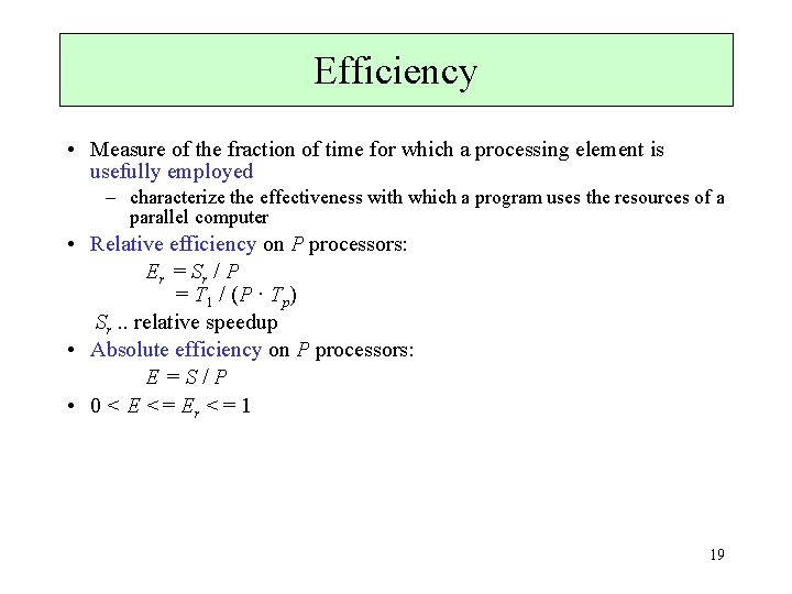
Efficiency • Measure of the fraction of time for which a processing element is usefully employed – characterize the effectiveness with which a program uses the resources of a parallel computer • Relative efficiency on P processors: Er = Sr / P = T 1 / (P · Tp) Sr. . relative speedup • Absolute efficiency on P processors: E=S/P • 0 < E <= Er <= 1 19

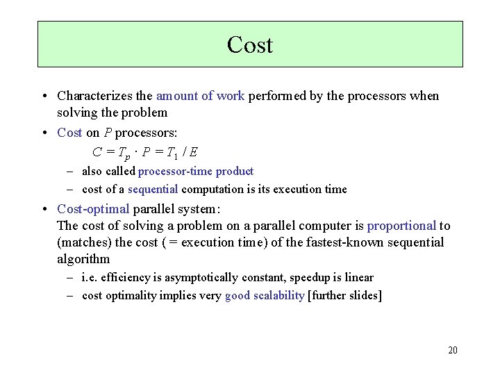
Cost • Characterizes the amount of work performed by the processors when solving the problem • Cost on P processors: C = Tp · P = T 1 / E – also called processor-time product – cost of a sequential computation is its execution time • Cost-optimal parallel system: The cost of solving a problem on a parallel computer is proportional to (matches) the cost ( = execution time) of the fastest-known sequential algorithm – i. e. efficiency is asymptotically constant, speedup is linear – cost optimality implies very good scalability [further slides] 20

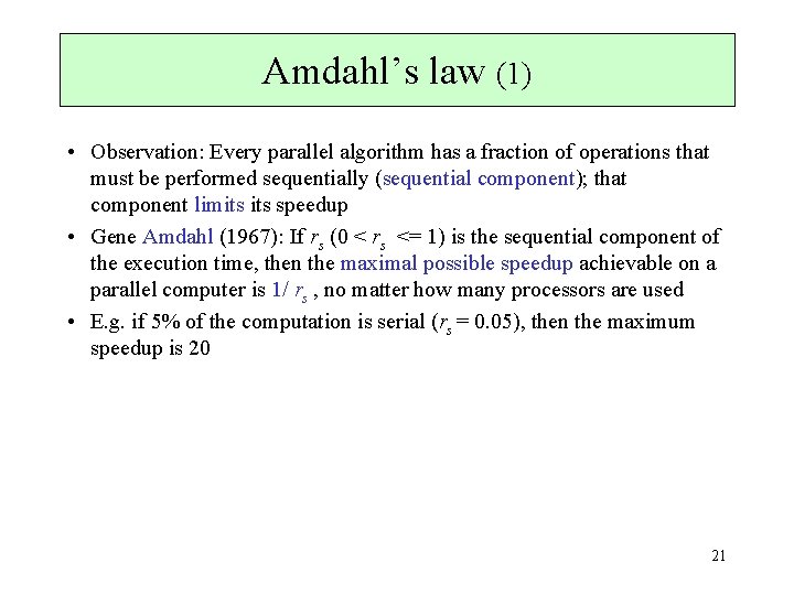
Amdahl’s law (1) • Observation: Every parallel algorithm has a fraction of operations that must be performed sequentially (sequential component); that component limits speedup • Gene Amdahl (1967): If rs (0 < rs <= 1) is the sequential component of the execution time, then the maximal possible speedup achievable on a parallel computer is 1/ rs , no matter how many processors are used • E. g. if 5% of the computation is serial (rs = 0. 05), then the maximum speedup is 20 21

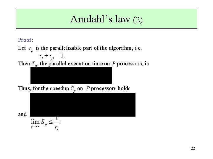
Amdahl’s law (2) Proof: Let rp is the parallelizable part of the algorithm, i. e. rs + rp = 1. Then Tp, the parallel execution time on P processors, is Thus, for the speedup Sp on P processors holds and 22

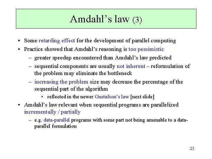
Amdahl’s law (3) • Some retarding effect for the development of parallel computing • Practice showed that Amdahl’s reasoning is too pessimistic – greater speedup encountered than Amdahl’s law predicted – sequential components are usually not inherent – reformulation of the problem may eliminate the bottleneck – increasing the problem size may decrease the percentage of the sequential part of the algorithm • reflected in the newer Gustafson’s law [next slide] • Amdahl’s law relevant when sequential programs are parallelized incrementally / partially – e. g. data-parallel programs with some part not being amenable to a dataparallel formulation 23

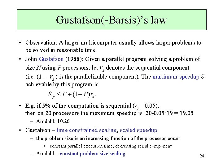
Gustafson(-Barsis)’s law • Observation: A larger multicomputer usually allows larger problems to be solved in reasonable time • John Gustafson (1988): Given a parallel program solving a problem of size N using P processors, let rs denotes the sequential component (i. e. (1 – rs ) is the parallelizable component). The maximum speedup S achievable by this program is • E. g. if 5% of the computation is sequential (rs = 0. 05), then on 20 processors the maximum speedup is 20 -0. 05· 19 = 19. 05 – Amdahl: 10. 26 • Gustafson – time constrained scaling, scaled speedup – the problem size is an increasing function of the processor count • constant parallel execution time, decreasing serial component – Amdahl – constant problem size scaling 24

Quantitative analysis • Investigates the adaptability of the parallel system to changes in the computing environment – problem size, number of processors, communication speed, memory size, etc. • Based on substitution of machine-specific numeric values for the various parameters in performance models – caution necessary – performance models are idealizations of complex phenomena • Most interesting: the ability to utilize increasing number of processors – studied in scalability analysis [next slides] 25

Scalability • Scalability of a parallel system is a measure of its ability to increase performance (speedup) as the number of processors increases – hardware scalability: the parallel computer can incorporate more processors without degrading the communication subsystem • Naively, one would assume that more processors (automatically) improve performance • Definition of a scalable parallel program (system) varies in literature; often imprecise formalization – e. g. “a parallel system is scalable if the performance is linearly proportional to the number of processors used ” 26

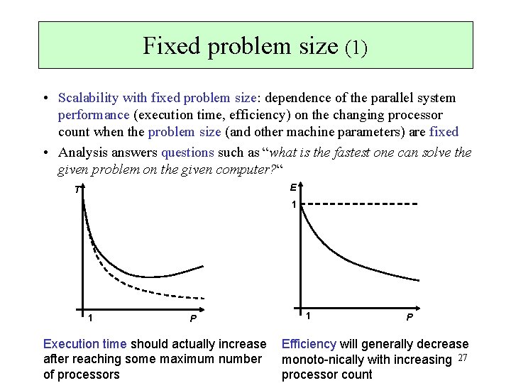
Fixed problem size (1) • Scalability with fixed problem size: dependence of the parallel system performance (execution time, efficiency) on the changing processor count when the problem size (and other machine parameters) are fixed • Analysis answers questions such as “what is the fastest one can solve the given problem on the given computer? “ E T 1 1 P Execution time should actually increase after reaching some maximum number of processors 1 P Efficiency will generally decrease monoto-nically with increasing 27 processor count

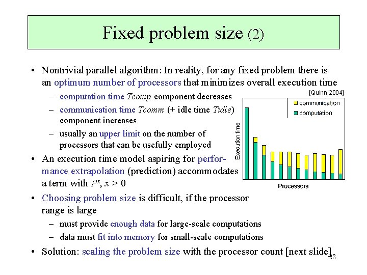
Fixed problem size (2) • Nontrivial parallel algorithm: In reality, for any fixed problem there is an optimum number of processors that minimizes overall execution time – computation time Tcomponent decreases – communication time Tcomm (+ idle time Tidle) component increases – usually an upper limit on the number of processors that can be usefully employed [Quinn 2004] • An execution time model aspiring for performance extrapolation (prediction) accommodates a term with Px, x > 0 • Choosing problem size is difficult, if the processor range is large – must provide enough data for large-scale computations – data must fit into memory for small-scale computations • Solution: scaling the problem size with the processor count [next slide]28

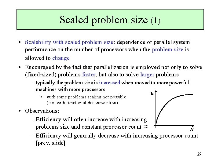
Scaled problem size (1) • Scalability with scaled problem size: dependence of parallel system performance on the number of processors when the problem size is allowed to change • Encouraged by the fact that parallelization is employed not only to solve (fixed-sized) problems faster, but also to solve larger problems – typically the problem size is increased when moved to more powerful machines with more processors • with some problems scaling not possible (e. g. with functional decomposition) E • Observations: – Efficiency will often increase with increasing problems size and constant processor count N – Efficiency will generally decrease with increasing processor count [prev. slide] 29

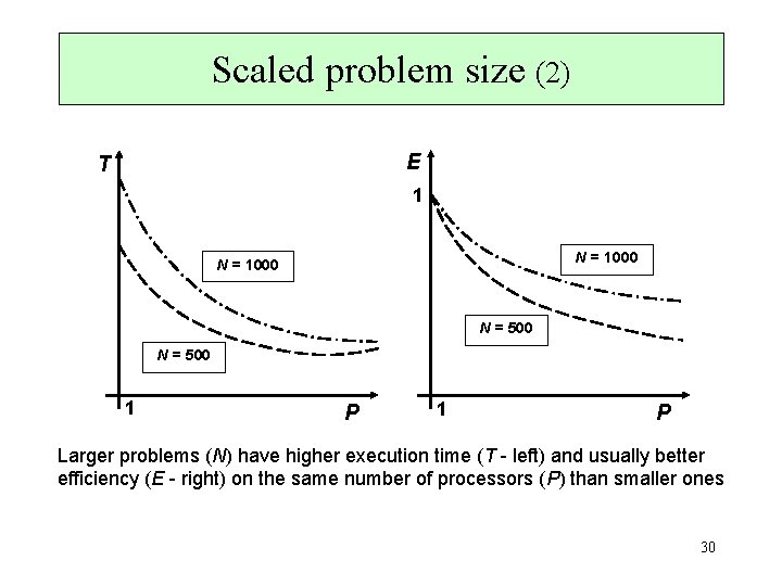
Scaled problem size (2) E T 1 N = 1000 N = 500 1 P Larger problems (N) have higher execution time (T - left) and usually better efficiency (E - right) on the same number of processors (P) than smaller ones 30

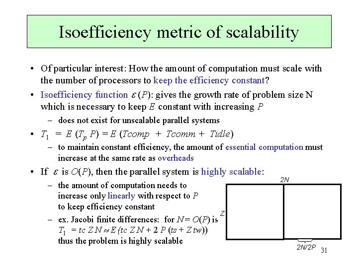
Isoefficiency metric of scalability • Of particular interest: How the amount of computation must scale with the number of processors to keep the efficiency constant? • Isoefficiency function (P): gives the growth rate of problem size N which is necessary to keep E constant with increasing P – does not exist for unscalable parallel systems • T 1 = E (Tp P) = E (Tcomp + Tcomm + Tidle) – to maintain constant efficiency, the amount of essential computation must increase at the same rate as overheads • If is O(P), then the parallel system is highly scalable: – the amount of computation needs to increase only linearly with respect to P to keep efficiency constant Z – ex. Jacobi finite differences: for N = O(P) is T 1 = tc Z N E (tc Z N + 2 P (ts + Z tw)) thus the problem is highly scalable 2 N 2 N/2 P 31

Other evaluation methods • Extrapolation from observations statements like “speedup of 10. 8 on 12 processors with problem size 100” small number of observations in a multidimensional space says little about the quality of the parallel system as a whole • Asymptotic analysis statements like “algorithm requires O(N log N) time on O(N) processors” deals with large N and P, usually out of scope of practical interest says nothing about absolute cost usually assumes idealized machine models (e. g. PRAM) more important for theory than practice 32

Conclusions • The lecture provides only with a “feel and taste“ introduction to the analytical modelling of parallel programs • Good knowledge required especially when supercomputing is concerned – practical experience from small parallel system is difficult to extrapolate to large problems targeted on machines with thousands of processors 33

Further study • Covered to some extent in all textbooks on parallel programming/computing – with attempts to specific point of view • The most profound coverage can be probably found in [Grama 2003] Introduction to Parallel Computing 34

35