Parallel Analysis of Algorithms PRAM CGM Outline Parallel

Parallel Analysis of Algorithms: PRAM + CGM

Outline Parallel Performance Parallel Models n n Shared Memory (PRAM, SMP) Distributed Memory (BSP, CGM) Parallel Analysis of Algorithms 2

Parallel Analysis of Algorithms Question? Professor speedy says he has a parallel algorithm for sorting n arbitrary items in n time using p>1 processors. Do you believe him? Parallel Analysis of Algorithms 3

Parallel Analysis of Algorithms Performance of a Parallel Algorithm n : p : T(p): Ts : s(p) = Ts problem size (e. g. : sort n numbers) number of processors parallel time sequential time (optimal sequ. alg. ) / T(p) : speedup (1 s p) s r a e n i s(p)=p l re p ar e su ar e lin in l sub p Parallel Analysis of Algorithms 4

Parallel Analysis of Algorithms Speedup linear speedup s(p) = p optimal super linear speedup s(p) > p : impossible Proof. Assume that parallel algorithm A has a speedup s > p for processors, i. e. s = Ts / T > p. Hence: Ts > T p. Simulate A on a sequential, single processor machine. Then T(1) = T · p < Ts. Hence, Ts was not optimal. Contradiction. Parallel Analysis of Algorithms 5

Parallel Analysis of Algorithms Amdahl’s Law Let f, 0<f<1, be the fraction of a computation that is inherently sequential. Then the maximum obtainable speedup is s <= 1 / [f+(1 -f)/p]. Proof: Ts = sequ. time. The T(p) f Ts + (1 -f)Ts / p. Hence s Ts / [f Ts +(1 -f) Ts /p] = 1 / [f+(1 -f)/p]. Parallel Analysis of Algorithms 6

Amdahl’s Law ts fts (1 - f)ts Serial section Parallelizable sections (a) One processor (b) Multiple processors p processors tp (1 - f)ts /p Parallel Analysis of Algorithms 7

Parallel Analysis of Algorithms Amdahl’s Law P=1 time P=5 P=10 Parallel Analysis of Algorithms P=1000 8

Parallel Analysis of Algorithms Amdahl’s Law s(p) 1 / [f+(1 -f)/p] f f 0 1 = 0. 5 = 1/k : : s (p) p s(p) 1 s(p) = 2 [p/(p+1)] <= 2 s(p) = k / [1+(k-1)/p] <= k Parallel Analysis of Algorithms 9

Parallel Analysis of Algorithms s k Parallel Analysis of Algorithms 10

Parallel Analysis of Algorithms Scaled or Relative Speedup Ts may be unknown (in fact, for most real experiments this is the case) Relative speedup s’ (p) = T(1) / T(p) s’ (p) s(p) Parallel Analysis of Algorithms 11

Parallel Analysis of Algorithms Efficiency e(p) = s(p) / p efficiency (0 e 1) optimal linear speedup s(p) = p e(p) = 1 e’(p) = s’(p) / p Relative efficiency Parallel Analysis of Algorithms 12

Outline Parallel Analysis of Algorithms Models n n Shared Memory (PRAM, SMP) Distributed Memory (BSP, CGM) Parallel Analysis of Algorithms 13

Shared Memory (PRAM, SMP) Parallel Random Access Machine (PRAM) Exclusive-Read (ER) Concurrent-Read (CR) proc. 1 proc. 2 1 2 proc. 3. . . Exclusive-Write (EW) Concurrent-Write (CW) shared memory proc. i j n-1 n . . . proc. p Parallel Analysis of Algorithms 14

Shared Memory (PRAM, SMP) Parallel Random Access Machine (PRAM) Concurrent-Write (CW) n Common: All proc. must write the same value n Arbitrary: An arbitrary value “wins” n Smallest: The smallest value “wins” n Priority: The proc. with smallest ID number “wins” proc. 1 proc. 2 shared memory 1 2 proc. 3. . . proc. i j n-1 n . . . proc. p Parallel Analysis of Algorithms 15

Shared Memory (PRAM, SMP) Parallel Random Access Machine (PRAM) Default: CREW (Concurrent Read Exclusive Write) proc. 1 proc. 2 shared memory 1 2 proc. 3 p = O(n) fine grained massively parallel . . . proc. i j n-1 n . . . proc. p Parallel Analysis of Algorithms 16

Shared Memory (PRAM, SMP) Performance of a PRAM Algorithm Optimal T = O ( Ts / p ) Efficient T = O ( logk(n) Ts / p ) NC T = O (logk(n) ) for p= polynomial (n) Parallel Analysis of Algorithms 17

Shared Memory (PRAM, SMP) Example: Multiply n numbers Input: a 1, a 2, …, an Output: a 1 * a 2 * a 3 * … * an * : associative operator proc. 1 proc. 2 shared memory 1 2 proc. 3. . . proc. i j n-1 n . . . proc. p Parallel Analysis of Algorithms 18

Shared Memory (PRAM, SMP) Algorithm 1 p = n/2 Parallel Analysis of Algorithms 19

Shared Memory (PRAM, SMP) Analysis p = n/2 T = O( log n ) Ts = O(n), Ts / p = O(1) algorithm is efficient & NC but not optimal Parallel Analysis of Algorithms 20

Shared Memory (PRAM, SMP) Algorithm 2 make available only p = n / log n processors execute Algorithm 1 using “rescheduling”: whenever Algorithm 1 has a parallel step where m > (n / log n) processors are used, simulate this step by a “phase” consisting of m / (n / log n) steps for (n / log n) processors Parallel Analysis of Algorithms 21

Shared Memory (PRAM, SMP) proc Parallel Analysis of Algorithms 22

Shared Memory (PRAM, SMP) Analysis # steps in phase i : (n / 2 i) / (n / log n) = log n / 2 i T = O( 1 i n log n / 2 i ) = O( log n 1 i n 1/ 2 i ) = O( log n ) p = n / log n Ts / p = O( n / [n / log n] ) = O( log n ) algorithm is efficient & NC & optimal Parallel Analysis of Algorithms 23

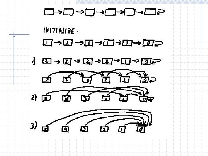
Problem 2: List Ranking Input: A linked list represented by an array. Output: The distance of each node to the last node.

Algorithm: Pointer Jumping Assign proc. i to node i Initialize (all proc. i in parallel): D(i) : = 0 if P(i)=i 1 otherwise REPEAT log n TIMES (all proc. i in parallel): D(i) : = D(i) + D(P(i)) P(i) : = P(P(i))

Analysis p=n T = O( log n ) efficient & NC but not optimal

Problem 3: Partial Sums Input: a 1, a 2, …, an Output: a 1 + a 2 + a 3. . . a 1 + a 2 + a 3 + … + a n

Parallel Recursion Compute (in parallel): a 1 + a 2 , a 3 + a 4 , a 5 + a 6 , . . . , an-1 + an Recursively (all proc. together) solve the problem for the n/2 numbers a 1 + a 2 , a 3 + a 4 , a 5 + a 6 , . . . , an-1 + an The result is: (a 1+a 2) (a 1+a 2+a 3+a 4+a 5+a 6 ) . . . (a 1+a 2. . . an-3+an 2) (a 1+a 2+an-1+an) Compute each gap by multiplying its predecessor by a single number

Analysis p=n T (n) = T(n/2) + O(1) T(1) = O(1) T(n) = O(log n) efficient and NC but not optimal

Improving through rescheduling set p = n / log n simulate previous algorithm

proc

Analysis # steps in phase i : (n / 2 i) / (n / log n) = log n / 2 i T = O( 1 i n log n / 2 i ) = O( log n 1 i n 1/ 2 i ) = O( log n ) p = n / log n Ts / p = O( n / [n / log n] ) = O( log n ) algorithm is efficient & NC & optimal

Problem 4: Sorting Input: a 1, a 2, …, an Output: a 1, a 2, …, an permuted into sorted order proc. 1 proc. 2 shared memory 1 2 proc. 3. . . proc. i. . . proc. p j n-1 n

Bitonic Sorting (Batcher) Unimodal sequence: 9 10 13 17 21 19 16 15 Bitonic sequence: cyclic shift of a unimodal sequence 16 15 9 10 13 17 21 19

Properties of bitonic sequences X = x 1 x 2. . . xn xn+1 xn+2. . . x 2 n bitonic L(X) = y 1. . . yn yi = min {xi, xn+i} U(X) = z 1. . . zn zi = max {xi, xn+i} (1) L(X) and U(X) are bitonic (2) every element of L(X) is smaller than every element of U(X).

Bitonic Merge: sorting a bitonic sequence of length n can be sorted in time O(log n) using p=n processors

sorting an arbitrary sequence a 1, a 2, …, an split a 1, a 2, …, an into two sub-sequences: a 1, …, an/2 and a(n/2)+1, a(n/2)+2, …, an recursively, in parallel, sort each subsequence using p/2 processors merge the two sorted sub-sequences into one sorted sequence using bitonic merge Note: If X and Y are sorted sequences (increasing order), then X YR is a bitonic sequence.

Analysis p=n T (n) = T(n/2) + O(log n) T(1) = O(1) T(n) = O(log 2 n) efficient and NC but not optimal

So what about a SMP machine? PRAM? n n n EREW? CRCW? How does Open. MP play into this? Parallel Analysis of Algorithms 40

Open. MP/SMP = CREW PRAM but coarse grained T(p) f Ts + (1 -f)Ts / p, for f = sequential fraction T(n, p) = f Ts + sum over all parallel regions of max time fork Master Thread Parallel Regions Parallel Analysis of Algorithms 41

Outline Parallel Analysis of Algorithms Models n n Shared Memory (PRAM, SMP) Distributed Memory (BSP, CGM) Parallel Analysis of Algorithms 42

Distributed Memory Models

Parallel Computing p: # processors n: problem size Ts(n): sequential time T(p, n): parallel time speedup: S(p, n) = Ts(n) / T(p, n) Goal: obtain linear speedup S(p, n)=p

Parallel Computers Beowulf Cluster Blue Gene/Q . . . Custom MPP (Tianhe-2) Cray XK 7

Parallel Machine Models How to abstract the machine into a simplified model such that n n algorithm/application design is not hampered by too many details calculated time complexity predictions match the actually observed running times (with sufficient accuracy)

Parallel Machine Models PRAM Fine grained networks (array, ring, mesh, hypercube) Bulk Synchronous Parallelism (BSP), Valiant, 1990 Coarse Grained Multicomputer (CGM), Dehne, Rau-Chaplin, 1993 Multithread (CILK), Leiserson, 1995 many more. . .

PRAM p=O(n) processors massively parallel. . .

Example: PRAM Sort list merge… Bitonic Sort: O(log n) per merge => O(log 2 n) Cole: O(1) per merge => O(log n)

Fine Grained Networks p=O(n) processors massively parallel. . .

Example: Mesh Sort O(n 1/2) time sub mesh merge

Back to reality. . . Would anyone use a parallel machine with n processors in order to sort n items ? Of course NOT… Typical parallel machines have large ratios n/p (e. g. n/p = 16 M)

Brent's Theorem Mapping: Fine grained => Coarse grained. Via virtual processors If we simulate n virtual processors on p real processors then S(p) = S(n) * p/n S(n)=O(n) "optimal" => S(p)=O(p) "optimal"

The Problem! • Fine Grained PRAM and Fixed Network algorithms are VERY slow when implemented on commercial parallel machines.

Why ?

Why ? S(p) P=n

Why ? n 1/2 S(n) = n log n / n 1/2 The assumption is not true: in most cases, S(n) is NOT optimal

CGM Coarse Grained Multicomputer Dehne, Rau-Chaplin, 1993 S(p) p=n p

CGM Coarse Grained Multicomputer Coarse grained memory Coarse grained computation Coarse grained communication

Coarse Grained Memory Ignore small n/p e. g. assume n/p > p

Coarse Grained Compute in supersteps with barrier synchronization (as in BSP)

Coarse Grained Comm. • All communication steps are h-relations, h=O(n/p) • No individual messages h-relation

h-Relation

CGM Coarse Grained Multicomputer • Complexity measure: – number of rounds (e. g. O(1), O(log p), …) – scalability (e. g. n/p > p) – local computation – communication volume

CGM Coarse Grained Multicomputer • Coarse grained memory • Coarse grained computation • Coarse grained communication => - practical parallel algorithms - efficient and portable

Det. Sample Sort CGM Algorithm: sort locally and create p-sample

Det. Sample Sort CGM Algorithm: • send all p-samples to processor 1

Det. Sample Sort CGM Algorithm: • proc. 1: sort all received samples and compute global p-sample

Det. Sample Sort CGM Algorithm: • broadcast global psample • bucket locally according to global p -sample • send bucket i to proc. i • resort locally

Det. Sample Sort CGM Algorithm: • O(1) rounds for n/p > p 2 • O(n/p log n) local comp. • Goodrich (FOCS'98): O(1) rounds for n/p > pe