Parallel Algorithms CS 170 Fall 2016 Parallel computation

Parallel Algorithms CS 170 Fall 2016

Parallel computation is here! • During your career, Moore’s Law will probably slow down a lot (possibly to a grinding halt…) • Google’s engine (reportedly) has about 900, 000 processors (recall Map-Reduce) • The fastest supercomputers have > 107 cores and 1017 -18 flops • So, in an Algorithms course we must at least mention parallel algorithms

This lecture • What are parallel algorithms, and how do they differ from (sequential) algorithms? • What are the important performance criteria parallel algorithms? • What are the basic tricks? • What does the “landscape” look like? • Sketches of two sophisticated parallel algorithms: MST and connected components

Parallel Algorithms need a completely new mindset!! In sequential algorithms: • We care about Time • Acceptable: O(n), O(n log n), O(n 2), O(|E||V|2)… • Polynomial time • Unacceptable: Exponential time 2 n • Sometimes unacceptable is the only possible: NP -complete problems • How about in parallel algorithms?

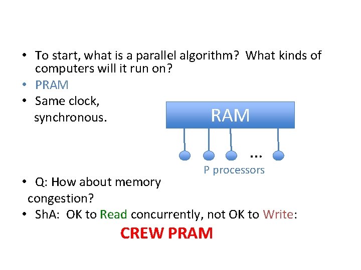
• To start, what is a parallel algorithm? What kinds of computers will it run on? • PRAM • Same clock, synchronous. RAM … P processors • Q: How about memory congestion? • Sh. A: OK to Read concurrently, not OK to Write: CREW PRAM

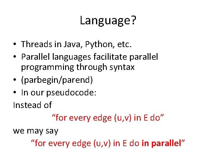
Language? • Threads in Java, Python, etc. • Parallel languages facilitate parallel programming through syntax • (parbegin/parend) • In our pseudocode: Instead of “for every edge (u, v) in E do” we may say “for every edge (u, v) in E do in parallel”

And what do we care about? • Two things: • Work = the total number of instructions executed by all processors • Depth = clock time in parallel execution

And what is acceptable? • Polynomial work • Depth? • O(log n) -- or maybe O((log n)2) etc. • Q: But how many processors? P = ? • A: Pretend to have as many as you want! • Saturate the problem with processors!

The reason: Brent’s Principle • If you can solve a problem with depth D and work W with as many processors as you want… • …then you can also solve it with P processors with work O(W) and depth D’ = D + W/P

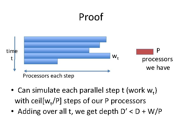
Proof time t wt P processors we have Processors each step • Can simulate each parallel step t (work wt) with ceil[wt/P] steps of our P processors • Adding over all t, we get depth D’ < D + W/P

To recap: Brent’s Principle If a problem can be solved in parallel with work W, depth D, and many processors, then it can be solved: • with P processors • the same work W’ = W • and depth D’ = W/P +D

Toy Problem: Sum Sequential algorithm sum = 0; for i = 1 to n do sum = sum + A[i] return sum O(n) time In parallel?

function sum(A[1. . n]) If n = 1 return A[1] for i = 1, …, n/2 do in parallel A[i] = A[2 i -1] + A[2 i] return sum(A[1. . n/2]) 23175486 5 8 9 14 13 23 36

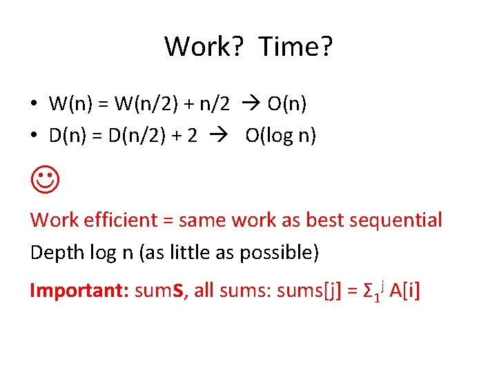
Work? Time? • W(n) = W(n/2) + n/2 O(n) • D(n) = D(n/2) + 2 O(log n) Work efficient = same work as best sequential Depth log n (as little as possible) Important: sums, all sums: sums[j] = Σ 1 j A[i]

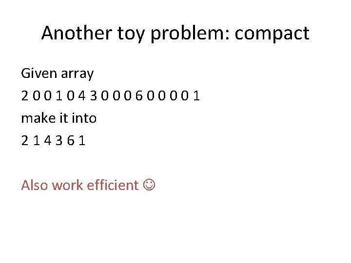
Another toy problem: compact Given array 2001043000600001 make it into 214361 Also work efficient

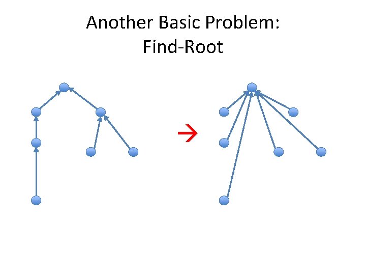
Another Basic Problem: Find-Root

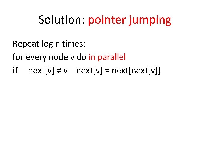
Solution: pointer jumping Repeat log n times: for every node v do in parallel if next[v] ≠ v next[v] = next[v]]

The parallel algorithm landscape • These are some of the very basic tricks of parallel algorithm design (like “divide and conquer” or “greedy” in algorithm design) • There a couple of others • The go a long way, but not all the way… • So, what happens to the problems we learned how to solve sequentially in CS 170?

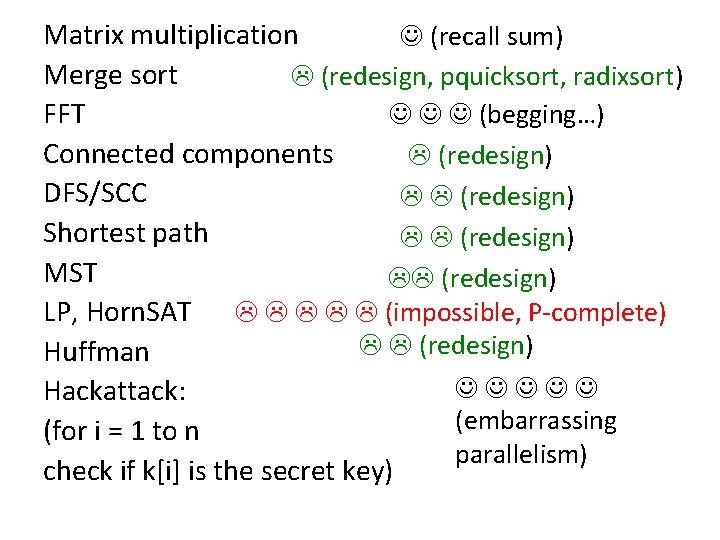
Matrix multiplication (recall sum) Merge sort (redesign, pquicksort, radixsort) (begging…) FFT Connected components (redesign) DFS/SCC (redesign) Shortest path (redesign) MST (redesign) LP, Horn. SAT (impossible, P-complete) (redesign) Huffman Hackattack: (embarrassing (for i = 1 to n parallelism) check if k[i] is the secret key)

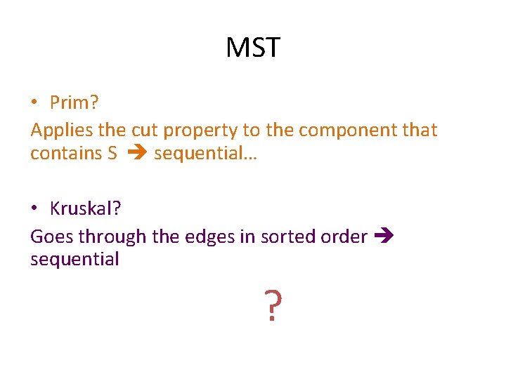
MST • Prim? Applies the cut property to the component that contains S sequential… • Kruskal? Goes through the edges in sorted order sequential ?

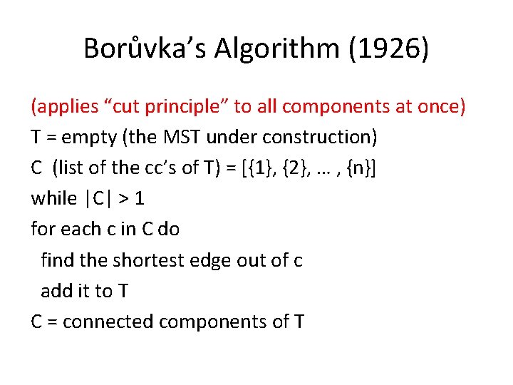
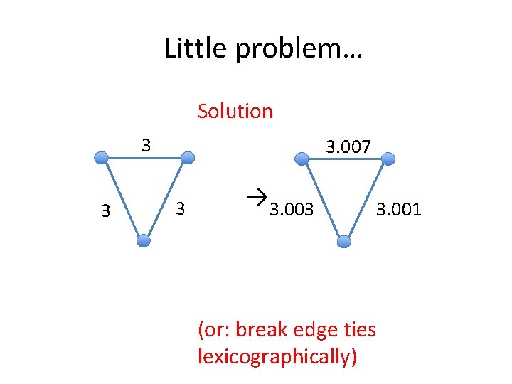
Borůvka’s Algorithm (1926) (applies “cut principle” to all components at once) T = empty (the MST under construction) C (list of the cc’s of T) = [{1}, {2}, … , {n}] while |C| > 1 for each c in C do find the shortest edge out of c add it to T C = connected components of T

Little problem… Solution 3 3 3. 007 3 3. 003 3. 001 (or: break edge ties lexicographically)

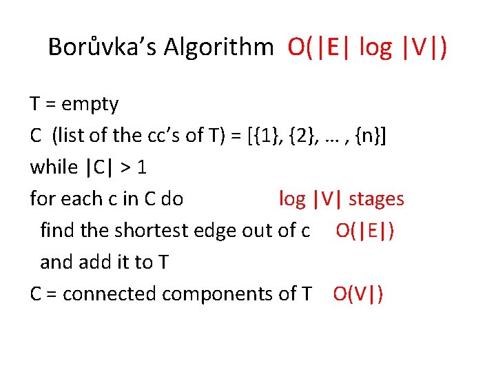
Borůvka’s Algorithm O(|E| log |V|) T = empty C (list of the cc’s of T) = [{1}, {2}, … , {n}] while |C| > 1 for each c in C do log |V| stages find the shortest edge out of c O(|E|) and add it to T C = connected components of T O(V|)

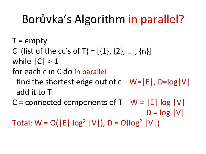
Borůvka’s Algorithm in parallel? T = empty C (list of the cc’s of T) = [{1}, {2}, … , {n}] while |C| > 1 for each c in C do in parallel find the shortest edge out of c W=|E|, D=log|V| add it to T C = connected components of T W = |E| log |V| D = log |V| Total: W = O(|E| log 2 |V|), D = O(log 2 |V|)

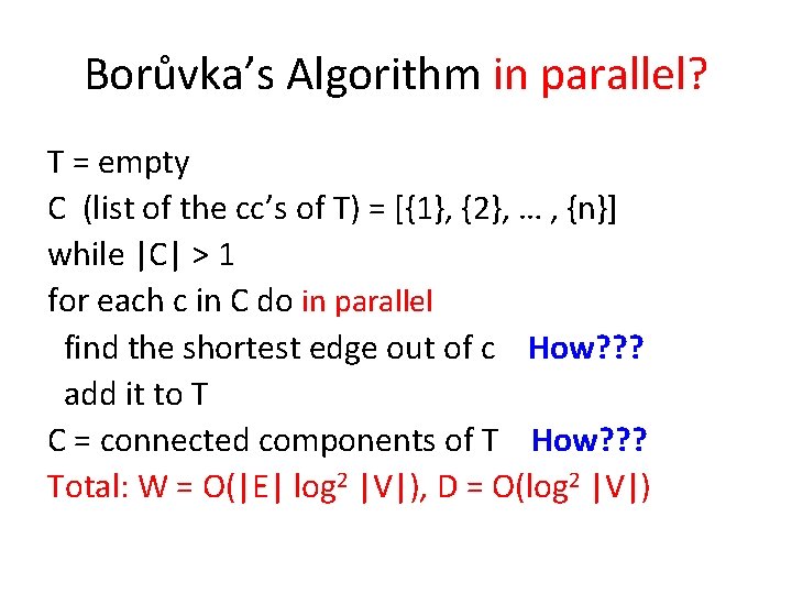
Borůvka’s Algorithm in parallel? T = empty C (list of the cc’s of T) = [{1}, {2}, … , {n}] while |C| > 1 for each c in C do in parallel find the shortest edge out of c How? ? ? add it to T C = connected components of T How? ? ? Total: W = O(|E| log 2 |V|), D = O(log 2 |V|)

Connected Components function cc(V, E) returns array[V] of V initialize: for every node v do in parallel: leader[v] = fifty-fifty(), ptr[v] = v for all non-leader node v do in parallel: chose an adjacent leader node u, if one exists, and set ptr[v] = u (ptr is now a bunch of stars) V’ = {v: ptr[v] = v} (the roots of the stars) E’ = {(u, v): u ≠ v in V’, there is (a, b) in E such that ptr[a] = u and ptr[b] = v} (“contract” the graph) label[] = cc(V’, E’) (compute cc recursively on the contracted graph) return cc[v] = label[ptr[v]]