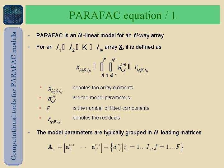
PARAFAC equation 1 PARAFAC is an N linear

PARAFAC equation / 1 • PARAFAC is an N -linear model for an N-way array • For an • array X, it is defined as § denotes the array elements § are the model parameters § F is the number of fitted components § denotes the residuals The model parameters are typically grouped in N loading matrices

HPLC-DAD Sulfonamide Interferent 0. 16 0. 12 Intensity [A. U. ] • HPLC combined with Diode Array Detection • Light absorbed at i-th wavelength 0. 08 0. 04 0 • Light absorbed at j-th time and i-th wavelength 25 50 Scan [ i - i ] 75 100 0 0. 2 Sulfonamide Interferent • For F compounds and K samples Intensity [A. U. ] 0. 15 0. 1 0. 05 0 240 280 320 360 l [nm] 400 440

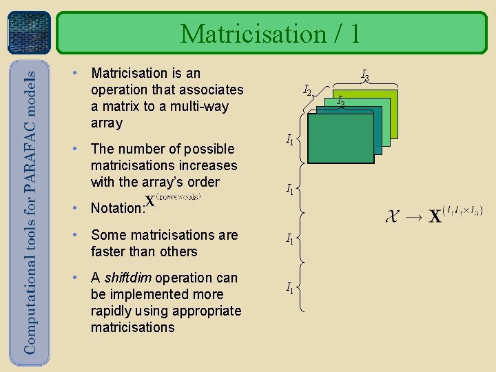
Matricisation / 1 • Matricisation is an operation that associates a matrix to a multi-way array • The number of possible matricisations increases with the array’s order I 2 I 1 • Notation: • Some matricisations are faster than others • A shiftdim operation can be implemented more rapidly using appropriate matricisations I 1 I 3

Matricisation / 1 I 1 • Matricisation is an operation that associates a matrix to a multi-way array • The number of possible matricisations increases with the array’s order I 2 I 1 I 2 • Notation: • Some matricisations are faster than others • A shiftdim operation can be implemented more rapidly using appropriate matricisations I 2 I 3

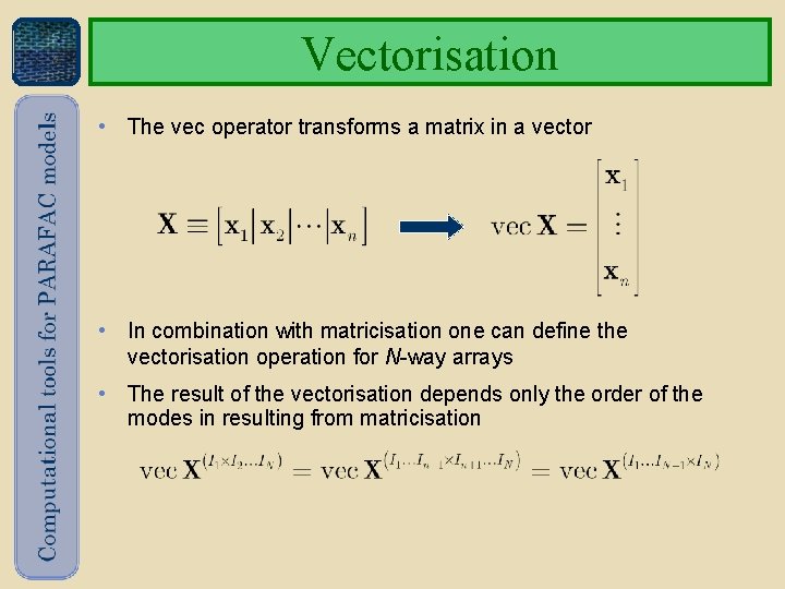
Vectorisation • The vec operator transforms a matrix in a vector • In combination with matricisation one can define the vectorisation operation for N-way arrays • The result of the vectorisation depends only the order of the modes in resulting from matricisation

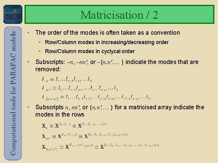
Matricisation / 2 • The order of the modes is often taken as a convention § Row/Column modes in increasing/decreasing order § Row/Column modes in cyclycal order • Subscripts: –n, –nn', or –{n, n', } indicate the modes that are removed: • Subscripts n, nn', or {n, n', } for a matricised array indicate the modes in the rows

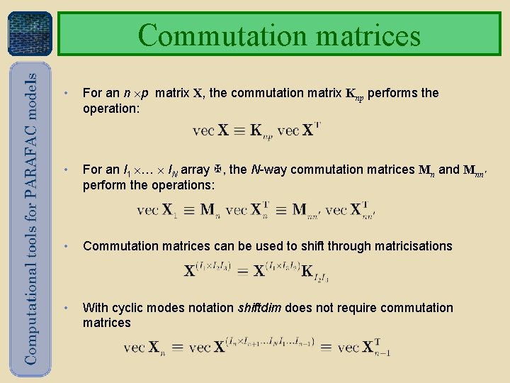
Commutation matrices • For an n p matrix X, the commutation matrix Knp performs the operation: • For an I 1 … IN array , the N-way commutation matrices Mn and Mnn' perform the operations: • Commutation matrices can be used to shift through matricisations • With cyclic modes notation shiftdim does not require commutation matrices

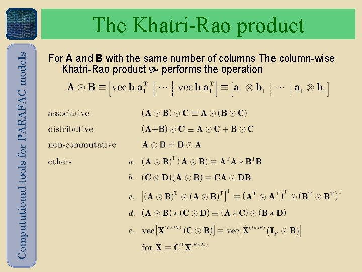
The Khatri-Rao product For A and B with the same number of columns The column-wise Khatri-Rao product performs the operation

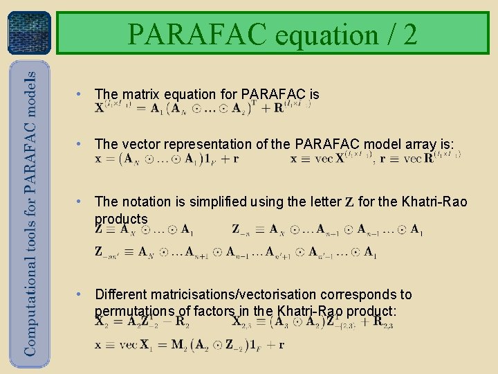
PARAFAC equation / 2 • The matrix equation for PARAFAC is • The vector representation of the PARAFAC model array is: • The notation is simplified using the letter Z for the Khatri-Rao products • Different matricisations/vectorisation corresponds to permutations of factors in the Khatri-Rao product:

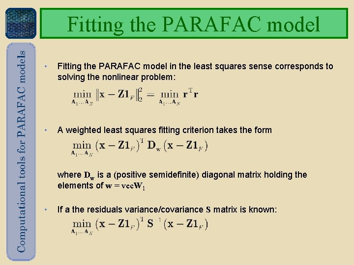
Fitting the PARAFAC model • Fitting the PARAFAC model in the least squares sense corresponds to solving the nonlinear problem: • A weighted least squares fitting criterion takes the form where Dw is a (positive semidefinite) diagonal matrix holding the elements of w = vec. W 1 • If a the residuals variance/covariance S matrix is known:

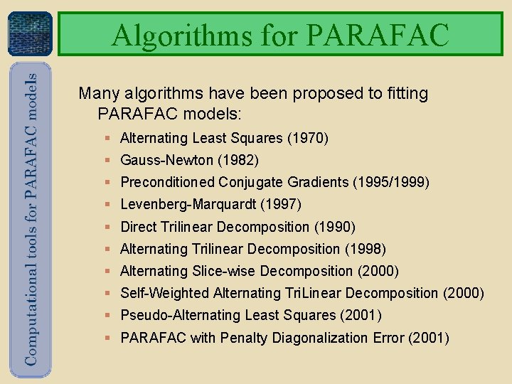
Algorithms for PARAFAC Many algorithms have been proposed to fitting PARAFAC models: § Alternating Least Squares (1970) § Gauss-Newton (1982) § Preconditioned Conjugate Gradients (1995/1999) § Levenberg-Marquardt (1997) § Direct Trilinear Decomposition (1990) § Alternating Trilinear Decomposition (1998) § Alternating Slice-wise Decomposition (2000) § Self-Weighted Alternating Tri. Linear Decomposition (2000) § Pseudo-Alternating Least Squares (2001) § PARAFAC with Penalty Diagonalization Error (2001)

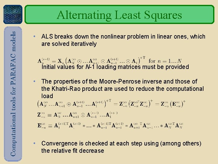
Alternating Least Squares • ALS breaks down the nonlinear problem in linear ones, which are solved iteratively Initial values for N-1 loading matrices must be provided • The properties of the Moore-Penrose inverse and those of the Khatri-Rao product are used to reduce the computational load • Convergence is checked at each step using (among others) the relative fit decrease

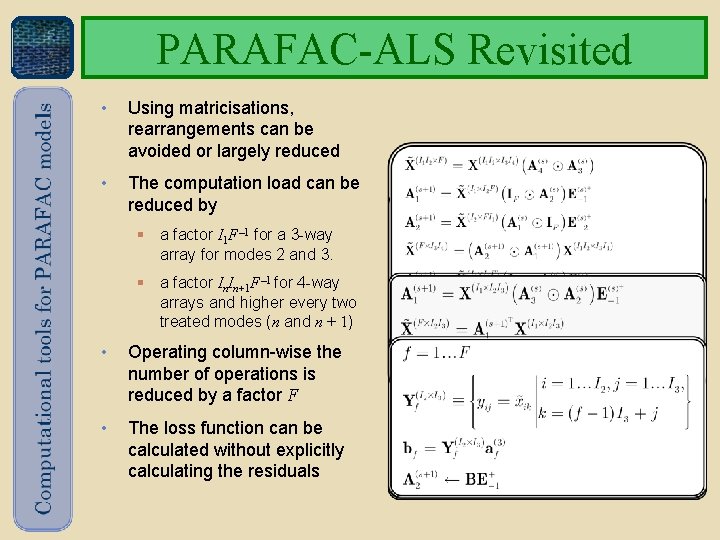
PARAFAC-ALS Revisited • Using matricisations, rearrangements can be avoided or largely reduced • The computation load can be reduced by § a factor I 1 F – 1 for a 3 -way array for modes 2 and 3. § a factor In. In+1 F – 1 for 4 -way arrays and higher every two treated modes (n and n + 1) • Operating column-wise the number of operations is reduced by a factor F • The loss function can be calculated without explicitly calculating the residuals

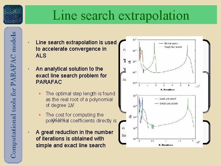
Line search extrapolation • Line search extrapolation is used to accelerate convergence in ALS • An analytical solution to the exact line search problem for PARAFAC § The optimal step length is found as the real root of a polynomial of degree 2 N. § The cost for computing the polynomial coefficients directly is • A great reduction in the number of iterations is obtained with simple and exact line search

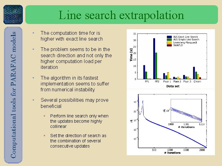
Line search extrapolation • The computation time for is higher with exact line search • The problem seems to be in the search direction and not only the higher computation load per iteration • The algorithm in its fastest implementation seems to suffer from numerical instability • Several possibilities may prove beneficial § Perform line search only when the updates become highly collinear § Set the direction of search as the combination of several consecutive updates

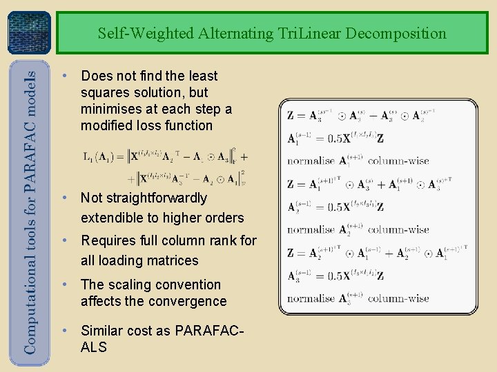
Self-Weighted Alternating Tri. Linear Decomposition • Does not find the least squares solution, but minimises at each step a modified loss function • Not straightforwardly extendible to higher orders • Requires full column rank for all loading matrices • The scaling convention affects the convergence • Similar cost as PARAFACALS

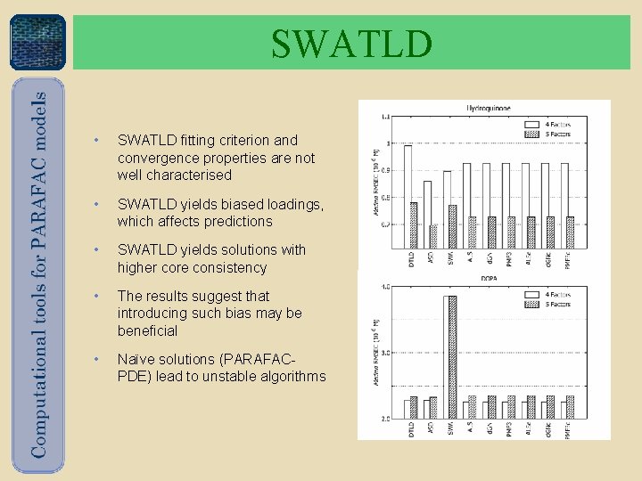
SWATLD • SWATLD fitting criterion and convergence properties are not well characterised • SWATLD yields biased loadings, which affects predictions • SWATLD yields solutions with higher core consistency • The results suggest that introducing such bias may be beneficial • Naïve solutions (PARAFACPDE) lead to unstable algorithms

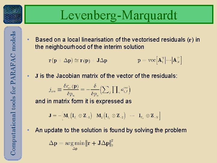
Levenberg-Marquardt • Based on a local linearisation of the vectorised residuals (r) in the neighbourhood of the interim solution • J is the Jacobian matrix of the vector of the residuals: and in matrix form it is expressed as • An update to the solution is found by solving the problem

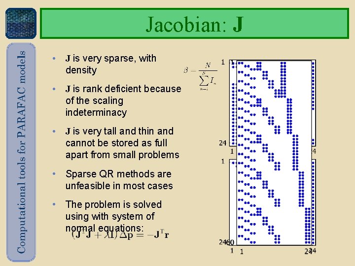
Jacobian: J • J is very sparse, with density • J is rank deficient because of the scaling indeterminacy • J is very tall and thin and cannot be stored as full apart from small problems • Sparse QR methods are unfeasible in most cases • The problem is solved using with system of normal equations:

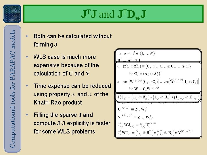
JTJ and JTDw. J • Both can be calculated without forming J • WLS case is much more expensive because of the calculation of U and V • Time expense can be reduced using property e. and c. of the Khatri-Rao product • Filling the sparse J and compute JTJ explicitly is faster for some WLS problems

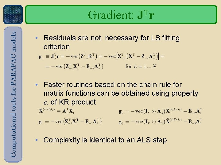
Gradient: JTr • Residuals are not necessary for LS fitting criterion • Faster routines based on the chain rule for matrix functions can be obtained using property e. of KR product • Complexity is identical to an ALS step

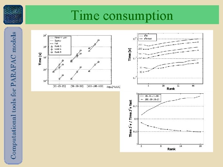
Time consumption

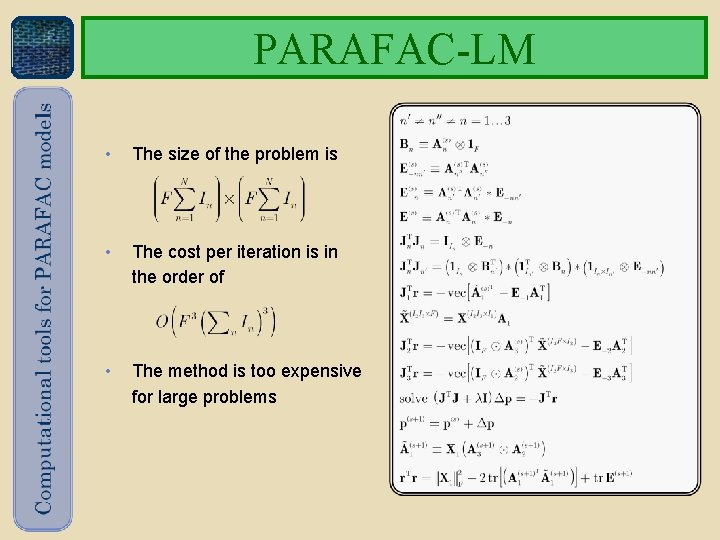
PARAFAC-LM • The size of the problem is • The cost per iteration is in the order of • The method is too expensive for large problems

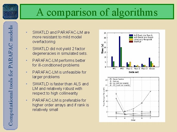
A comparison of algorithms • SWATLD and PARAFAC-LM are more resistant to mild model overfactoring • SWATLD did not yield 2 factor degeneracies in simulated sets. • PARAFAC-LM performs better for ill-conditioned problems • PARAFAC-LM is unfeasible for larger problems • SWATLD is faster than ALS and LM and relatively robust with respect to high collinearity • PARAFAC-LM is preferable for higher order arrays and if rank is relatively small

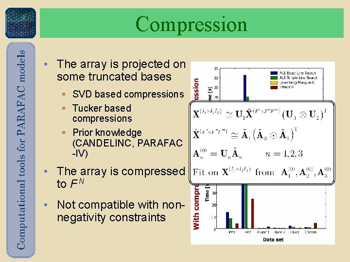
Compression • The array is projected on some truncated bases § SVD based compressions § Tucker based compressions § Prior knowledge (CANDELINC, PARAFAC -IV) • The array is compressed to F N • Not compatible with nonnegativity constraints

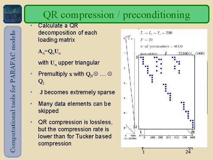
QR compression / preconditioning • Calculate a QR decomposition of each loading matrix An=Qn. Un with Un upper triangular • Premultiply x with QN Q 1 • J becomes extremely sparse • Many data elements can be skipped • QR compression is lossless, but the compression rate is lower than for Tucker based compression

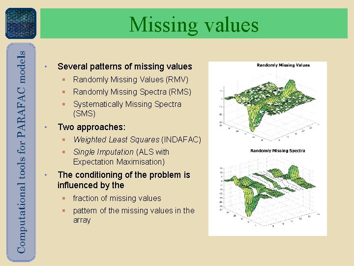
Missing values • Several patterns of missing values § Randomly Missing Values (RMV) § Randomly Missing Spectra (RMS) § Systematically Missing Spectra (SMS) • Two approaches: § Weighted Least Squares (INDAFAC) § Single Imputation (ALS with Expectation Maximisation) • The conditioning of the problem is influenced by the § fraction of missing values § pattern of the missing values in the array

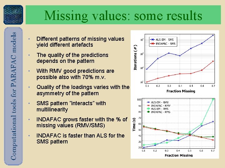
Missing values: some results • Different patterns of missing values yield different artefacts • The quality of the predictions depends on the pattern • With RMV good predictions are possible also with 70% m. v. • Quality of the loadings varies with the asymmetry of the pattern • SMS pattern ”interacts” with multilinearity • INDAFAC grows faster with the % of missing values (RMV/SMS) • INDAFAC is faster than ALS for the SMS pattern

Final remarks • There appears to be no method superior to any other in all conditions • There is great need for numerical insight in the algorithms. Faster algorithms may entail numerical instability • Several properties of the column-wise Khatri-Rao product can be used to reduce the computation load • Numerous methods have not been investigated yet 30