Panel and Time Series Cross Section Models Sociology

Panel and Time Series Cross Section Models Sociology 229: Advanced Regression Copyright © 2010 by Evan Schofer Do not copy or distribute without permission

Announcements • Assignment 5 Due • Assignment 6 handed out

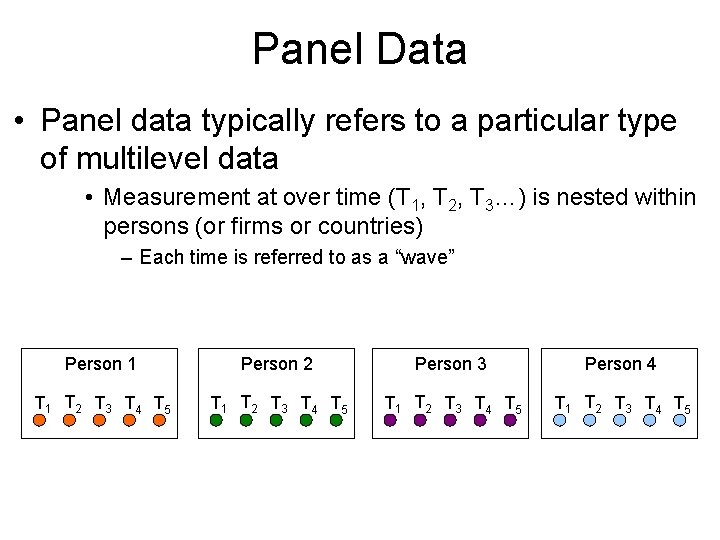
Panel Data • Panel data typically refers to a particular type of multilevel data • Measurement at over time (T 1, T 2, T 3…) is nested within persons (or firms or countries) – Each time is referred to as a “wave” Person 1 Person 2 Person 3 Person 4 T 1 T 2 T 3 T 4 T 5

Panel Data • Panel data involves combining: • Information about multiple cases – A “cross-sectional” component • Information about cases over time – A ‘longitudinal’ or ‘time series’ component • Panel datasets are described in terms of: • N, the number of individual cases • T, the number of waves – If N is “large” compared to T, the dataset is called “crosssectionally dominant” – If T is “large” compared to N, the dataset is called “timeseries dominant” • “Time-series Cross-section” / TSCS data: small set of units (usually 10 -30), moderate T

Panel Terminology • Issue: Panel means 2 things: • 1. Panel is an umbrella term for all data with timeseries and cross-section components • 2. Panel refers specifically to datasets with large N, small T (cross-sectionally dominant) – Example: a survey of 1000 people at 3 points in time – Another distinction: Balanced vs unbalanced • Panel data are said to be “balanced” if information on each person is available for all T • If data is missing for some cases at some points in time, the data are “unbalanced” – This is common for many datasets on countries or firms.

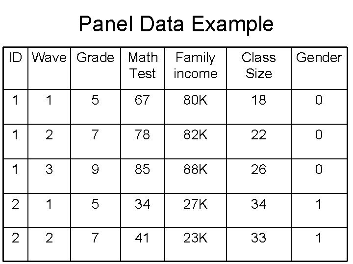
Panel Data Example ID Wave Grade Math Test Family income Class Size Gender 1 1 5 67 80 K 18 0 1 2 7 78 82 K 22 0 1 3 9 85 88 K 26 0 2 1 5 34 27 K 34 1 2 2 7 41 23 K 33 1

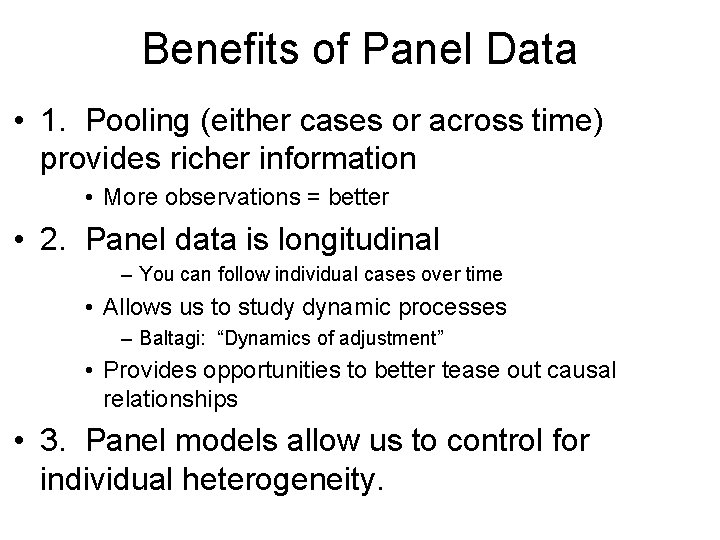
Benefits of Panel Data • 1. Pooling (either cases or across time) provides richer information • More observations = better • 2. Panel data is longitudinal – You can follow individual cases over time • Allows us to study dynamic processes – Baltagi: “Dynamics of adjustment” • Provides opportunities to better tease out causal relationships • 3. Panel models allow us to control for individual heterogeneity.

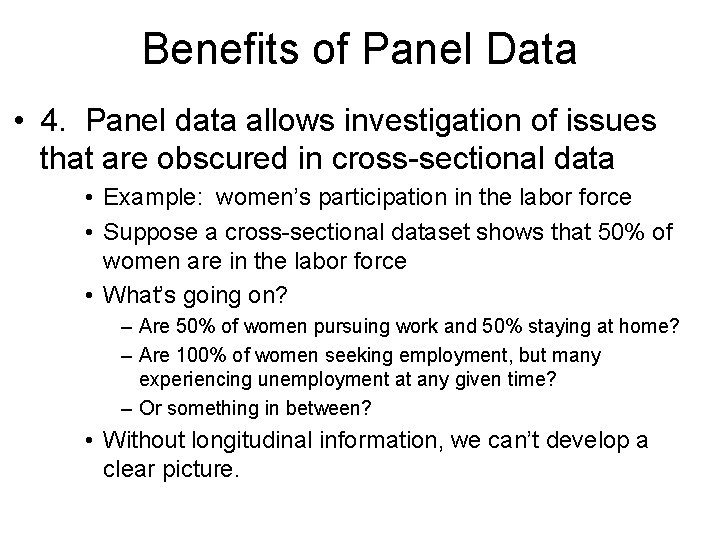
Benefits of Panel Data • 4. Panel data allows investigation of issues that are obscured in cross-sectional data • Example: women’s participation in the labor force • Suppose a cross-sectional dataset shows that 50% of women are in the labor force • What’s going on? – Are 50% of women pursuing work and 50% staying at home? – Are 100% of women seeking employment, but many experiencing unemployment at any given time? – Or something in between? • Without longitudinal information, we can’t develop a clear picture.

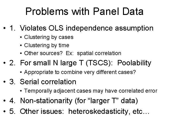
Problems with Panel Data • 1. Violates OLS independence assumption • Clustering by cases • Clustering by time • Other sources? Ex: spatial correlation • 2. For small N large T (TSCS): Poolability • Appropriate to combine very different cases? • 3. Serial correlation • Temporally adjacent cases may have correlated error • 4. Non-stationarity (for “larger T” data) • 5. Other issues: heteroskedasticity, etc…

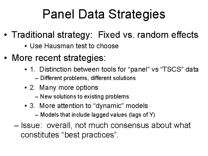
Panel Data Strategies • Traditional strategy: Fixed vs. random effects • Use Hausman test to choose • More recent strategies: • 1. Distinction between tools for “panel” vs “TSCS” data – Different problems, different solutions • 2. Many more options – New solutions to existing problems • 3. More attention to “dynamic” models – Models that include lagged values (lags of Y) – Issue: overall, not much consensus about what constitutes “best practices”.

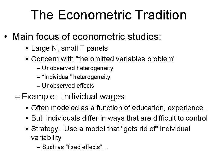
The Econometric Tradition • Main focus of econometric studies: • Large N, small T panels • Concern with “the omitted variables problem” – Unobserved heterogeneity – “Individual” heterogeneity – Unobserved effects – Example: Individual wages • Often modeled as a function of education, experience. . . • But, individuals differ in ways that are difficult to control • Strategy: Use a model that “gets rid of” individual variability – Such as “fixed effects”…

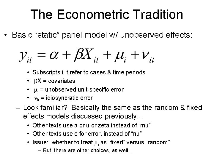
The Econometric Tradition • Basic “static” panel model w/ unobserved effects: • • Subscripts i, t refer to cases & time periods b. X = covariates mi = unobserved unit-specific error nit = idiosyncratic error – Look familiar? Basically the same as the random & fixed effects models discussed previously… • Other texts use a or u or zeta instead of “mu” • Other texts use e for error, instead of “nu” • Issue: whether to treat mi as “fixed” versus “random” – But, there are other choices, as well…

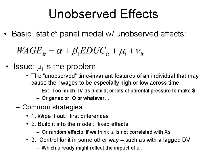
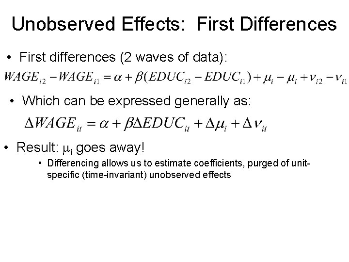
Unobserved Effects • Basic “static” panel model w/ unobserved effects: • Issue: mi is the problem • The “unobserved” time-invariant features of an individual that may cause their wages to be especially high or low across time – Ex: Too much TV as a child; or lots of parental pressure to make $ – Or genes or IQ or whatever… – Common strategies: • 1. Wipe it out: first differences • 2. Build it into the model: fixed effects – Or random effects, if we think mi is not correlated with Xs • 3. Control for it in some other way – such as with a lagged DV – Which already might reflect the impact of mi.

Unobserved Effects: First Differences • First differences (2 waves of data): • Which can be expressed generally as: • Result: mi goes away! • Differencing allows us to estimate coefficients, purged of unitspecific (time-invariant) unobserved effects

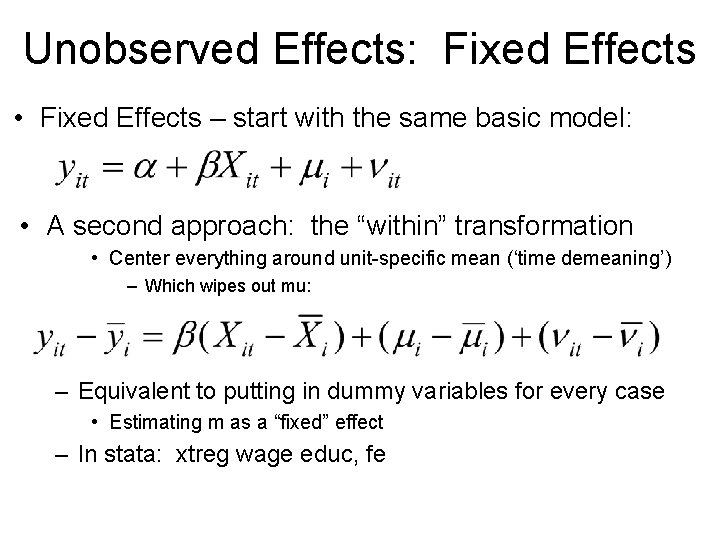
Unobserved Effects: Fixed Effects • Fixed Effects – start with the same basic model: • A second approach: the “within” transformation • Center everything around unit-specific mean (‘time demeaning’) – Which wipes out mu: – Equivalent to putting in dummy variables for every case • Estimating m as a “fixed” effect – In stata: xtreg wage educ, fe

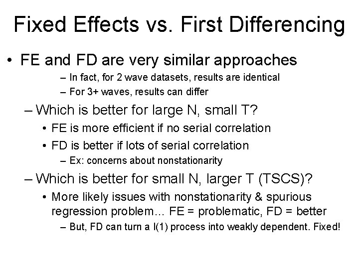
Fixed Effects vs. First Differencing • FE and FD are very similar approaches – In fact, for 2 wave datasets, results are identical – For 3+ waves, results can differ – Which is better for large N, small T? • FE is more efficient if no serial correlation • FD is better if lots of serial correlation – Ex: concerns about nonstationarity – Which is better for small N, larger T (TSCS)? • More likely issues with nonstationarity & spurious regression problem… FE = problematic, FD = better – But, FD can turn a I(1) process into weakly dependent. Fixed!

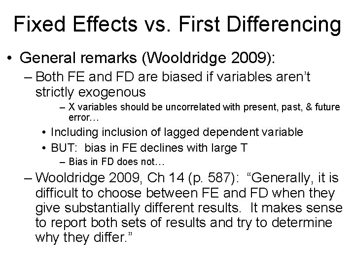
Fixed Effects vs. First Differencing • General remarks (Wooldridge 2009): – Both FE and FD are biased if variables aren’t strictly exogenous – X variables should be uncorrelated with present, past, & future error… • Including inclusion of lagged dependent variable • BUT: bias in FE declines with large T – Bias in FD does not… – Wooldridge 2009, Ch 14 (p. 587): “Generally, it is difficult to choose between FE and FD when they give substantially different results. It makes sense to report both sets of results and try to determine why they differ. ”

Fixed Effects vs. First Differencing • More remarks – 1. FE and FD cannot estimate effects of variables that do not change over time • And can have problems if variables change rarely… – 2. Both FE and FD are not as efficient as models that include “between case” variability • A trade off between efficiency and potential bias (if unobserved effects are correlated with Xs) – 3. Both FE and FD are very sensitive to measurement error • Within-case variability is often small… may be swamped by error/noise.

“Two-way” Error Components • Unobserved effects may occur over time – Example: common effect of year (e. g. , a recession) on wages • A “crossed” multilevel model • What Baltagi (2008) calls 2 -way error components – Versus basic FE/RE, which has one eror component – Strategies: • Use dummies for time in combination with FE/FD • Specify a “crossed” multilevel model in Stata – See Rabe-Hesketh and Skrondal – Basically, create a 3 -level model, nesting groups underneath.

Random Effects • Random effects: Additional efficiency at the cost of additional assumptions – Key assumption: unit-specific unobserved effect is not correlated with X variables – If assumptions aren’t met, results are biased • Omitted X variables often induce correlation between other X variables and the unobserved effect • If main purpose of panel analysis is to avoid unobserved effects, fixed effects is a safer choice – In stata: • xtreg wage educ, re – for GLS estimator • xtreg wage educ, mle – for ML estimator

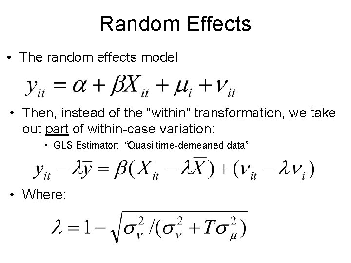
Random Effects • The random effects model • Then, instead of the “within” transformation, we take out part of within-case variation: • GLS Estimator: “Quasi time-demeaned data” • Where:

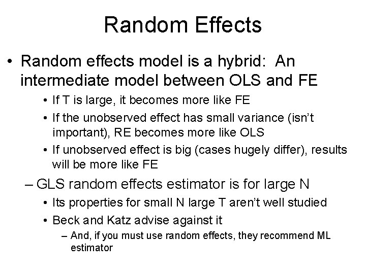
Random Effects • Random effects model is a hybrid: An intermediate model between OLS and FE • If T is large, it becomes more like FE • If the unobserved effect has small variance (isn’t important), RE becomes more like OLS • If unobserved effect is big (cases hugely differ), results will be more like FE – GLS random effects estimator is for large N • Its properties for small N large T aren’t well studied • Beck and Katz advise against it – And, if you must use random effects, they recommend ML estimator

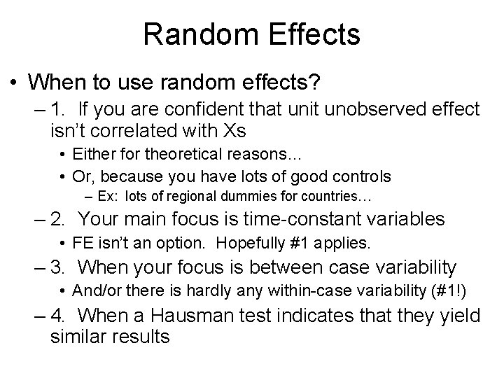
Random Effects • When to use random effects? – 1. If you are confident that unit unobserved effect isn’t correlated with Xs • Either for theoretical reasons… • Or, because you have lots of good controls – Ex: lots of regional dummies for countries… – 2. Your main focus is time-constant variables • FE isn’t an option. Hopefully #1 applies. – 3. When your focus is between case variability • And/or there is hardly any within-case variability (#1!) – 4. When a Hausman test indicates that they yield similar results

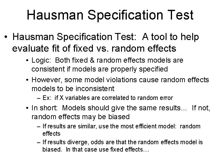
Hausman Specification Test • Hausman Specification Test: A tool to help evaluate fit of fixed vs. random effects • Logic: Both fixed & random effects models are consistent if models are properly specified • However, some model violations cause random effects models to be inconsistent – Ex: if X variables are correlated to random error • In short: Models should give the same results… If not, random effects may be biased – If results are similar, use the most efficient model: random effects – If results diverge, odds are that the random effects model is biased. In that case use fixed effects…

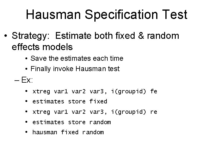
Hausman Specification Test • Strategy: Estimate both fixed & random effects models • Save the estimates each time • Finally invoke Hausman test – Ex: • • • xtreg var 1 var 2 var 3, i(groupid) fe estimates store fixed xtreg var 1 var 2 var 3, i(groupid) re estimates store random hausman fixed random

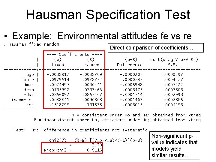
Hausman Specification Test • Example: Environmental attitudes fe vs re. hausman fixed random Direct comparison of coefficients… ---- Coefficients ---| (b) (B) (b-B) sqrt(diag(V_b-V_B)) | fixed random Difference S. E. -------+--------------------------------age | -. 0038917 -. 0038709 -. 0000207. 0000297 male |. 0979514. 0978732. 0000783. 0004277 dmar |. 0024493. 0030441 -. 0005948. 0007222 demp | -. 0733992 -. 0737466. 0003475. 0007303 educ |. 0856092. 0857407 -. 0001314. 0002993 incomerel |. 0088841. 0090308 -. 0001467. 0002885 ses |. 1318295. 131528. 0003015. 0004153 ---------------------------------------b = consistent under Ho and Ha; obtained from xtreg B = inconsistent under Ha, efficient under Ho; obtained from xtreg Test: Ho: difference in coefficients not systematic chi 2(7) = (b-B)'[(V_b-V_B)^(-1)](b-B) = 2. 70 Prob>chi 2 = 0. 9116 Non-significant pvalue indicates that models yield similar results…

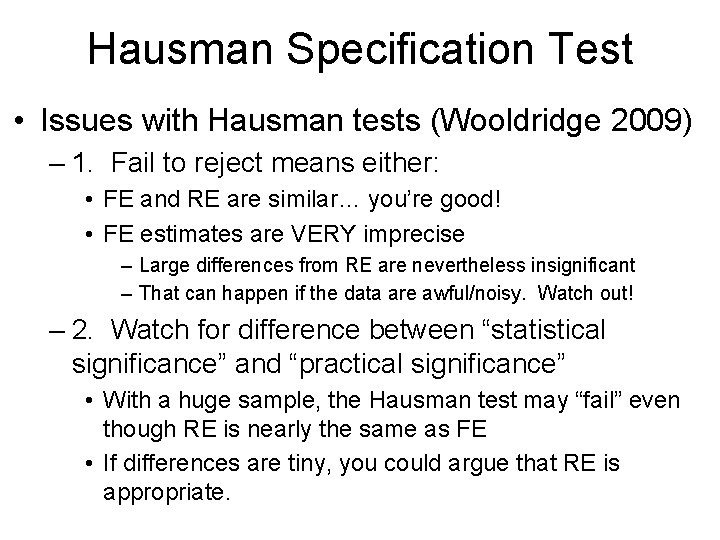
Hausman Specification Test • Issues with Hausman tests (Wooldridge 2009) – 1. Fail to reject means either: • FE and RE are similar… you’re good! • FE estimates are VERY imprecise – Large differences from RE are nevertheless insignificant – That can happen if the data are awful/noisy. Watch out! – 2. Watch for difference between “statistical significance” and “practical significance” • With a huge sample, the Hausman test may “fail” even though RE is nearly the same as FE • If differences are tiny, you could argue that RE is appropriate.

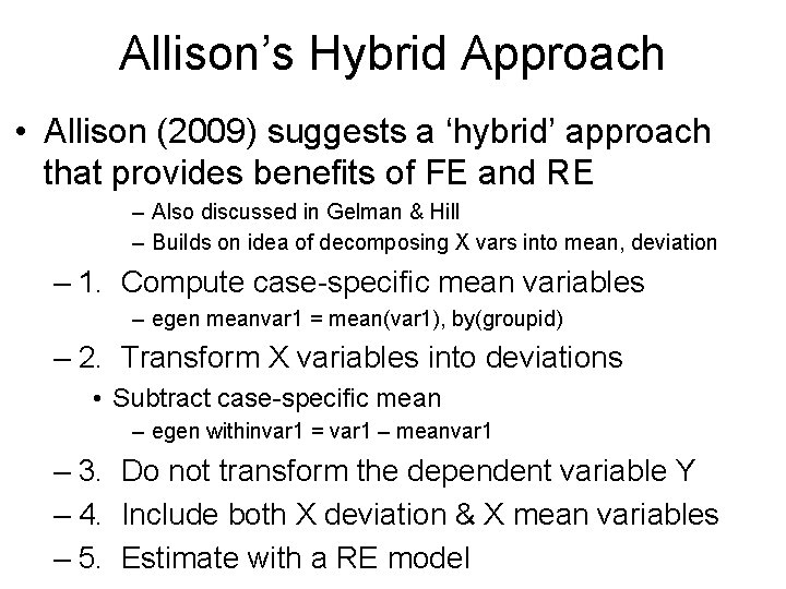
Allison’s Hybrid Approach • Allison (2009) suggests a ‘hybrid’ approach that provides benefits of FE and RE – Also discussed in Gelman & Hill – Builds on idea of decomposing X vars into mean, deviation – 1. Compute case-specific mean variables – egen meanvar 1 = mean(var 1), by(groupid) – 2. Transform X variables into deviations • Subtract case-specific mean – egen withinvar 1 = var 1 – meanvar 1 – 3. Do not transform the dependent variable Y – 4. Include both X deviation & X mean variables – 5. Estimate with a RE model

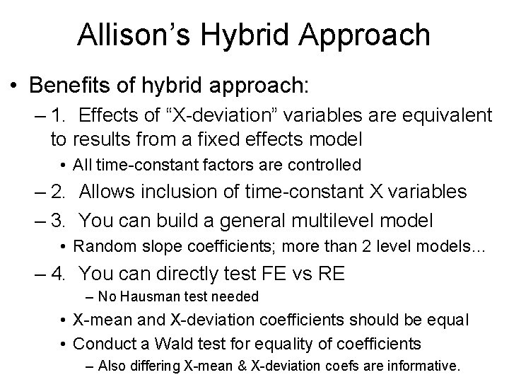
Allison’s Hybrid Approach • Benefits of hybrid approach: – 1. Effects of “X-deviation” variables are equivalent to results from a fixed effects model • All time-constant factors are controlled – 2. Allows inclusion of time-constant X variables – 3. You can build a general multilevel model • Random slope coefficients; more than 2 level models… – 4. You can directly test FE vs RE – No Hausman test needed • X-mean and X-deviation coefficients should be equal • Conduct a Wald test for equality of coefficients – Also differing X-mean & X-deviation coefs are informative.

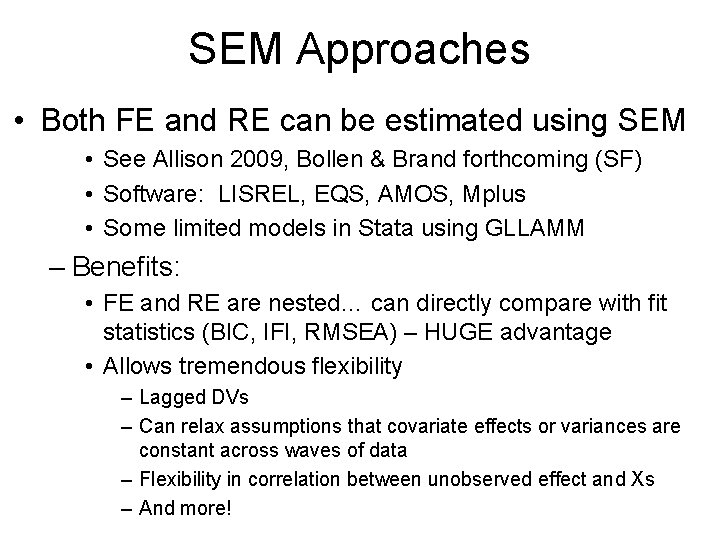
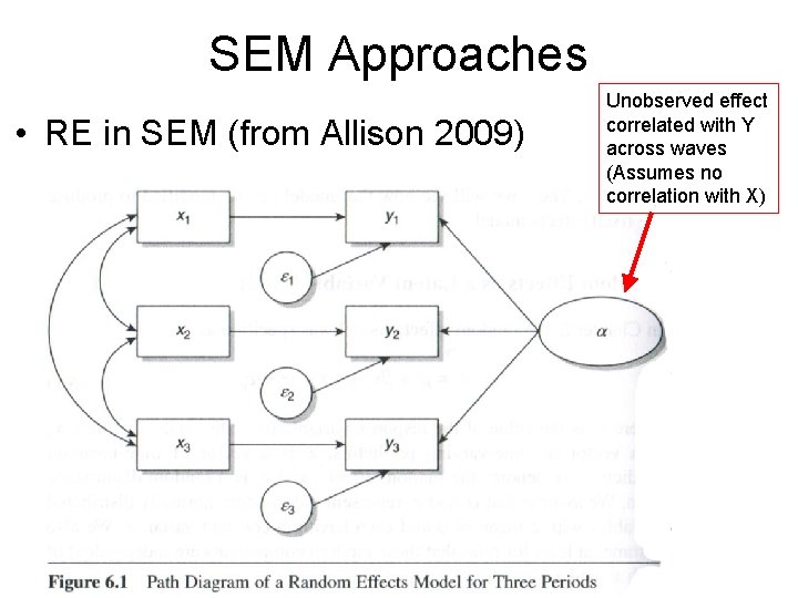
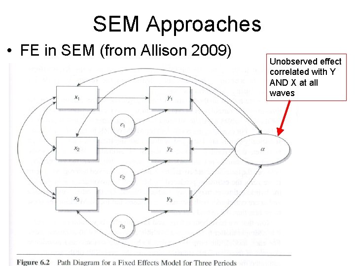
SEM Approaches • Both FE and RE can be estimated using SEM • See Allison 2009, Bollen & Brand forthcoming (SF) • Software: LISREL, EQS, AMOS, Mplus • Some limited models in Stata using GLLAMM – Benefits: • FE and RE are nested… can directly compare with fit statistics (BIC, IFI, RMSEA) – HUGE advantage • Allows tremendous flexibility – Lagged DVs – Can relax assumptions that covariate effects or variances are constant across waves of data – Flexibility in correlation between unobserved effect and Xs – And more!

SEM Approaches • RE in SEM (from Allison 2009) Unobserved effect correlated with Y across waves (Assumes no correlation with X)

SEM Approaches • FE in SEM (from Allison 2009) Unobserved effect correlated with Y AND X at all waves

Serial Correlation • Issue: What about correlated error in nearby waves of data? • So far we’ve focused on correlated error due to unobserved effect (within each case) – Strategies: – Use a model that accounts for serial correlation • STATA: xtregar – FE and RE with “AR(1) disturbance” – Many other options… xtgee, etc. – Develop a “dynamic model” • Actually model the patterns of correlation across Y – Include the lagged dependent variable (Y)… or many lags! • This causes bias in FE, RE – so other models needed.

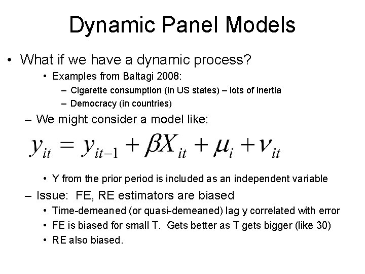
Dynamic Panel Models • What if we have a dynamic process? • Examples from Baltagi 2008: – Cigarette consumption (in US states) – lots of inertia – Democracy (in countries) – We might consider a model like: • Y from the prior period is included as an independent variable – Issue: FE, RE estimators are biased • Time-demeaned (or quasi-demeaned) lag y correlated with error • FE is biased for small T. Gets better as T gets bigger (like 30) • RE also biased.

Dynamic Panel Models • One solution: Use FD and instrumental variables – Strategy: If there’s a problem between error and lag Y, let’s find a way to calculate a NEW version of lag y that doesn’t pose a problem • Idea: Further lags of Y aren’t an issue in a FD model. • Use them as “instrumental variables” as a proxy for lag Y – Arellano Bond GMM estimator • A FD estimator • Lag of levels as an instrument for differenced Y – Arellano-Bover/Blundell-Bond “System GMM” estimator • Expand on this by using lags of differences and levels as instruments • Generalized Method of Moments (GMM) estimation.

Dynamic Panel Models • Stata: – xtabond – basic Arellano-Bond GMM model – xtdpdsys – System GMM estimator – xtdpd – A flexible command to build system GMM models • Lots of control over lag structure • Can run non-dynamic models – Key assumptions / issues – Serial correlation of differenced errors limited to 1 lag – No overidentifying restrictions (“Sargan test”) – How many instruments? – Criticisms: • Angrist & Pichke 2009: assumptions not always plausible • Allison 2009 • Bollen and Brand, forth: Hard to compare models.

Dynamic Panel Models • General remarks: – It is important to think carefully about dynamic processes… • How long does it take things to unfold? • What lags does it make sense to include? • With huge datasets, we can just throw lots in – With smaller datasets, it is important to think things through.

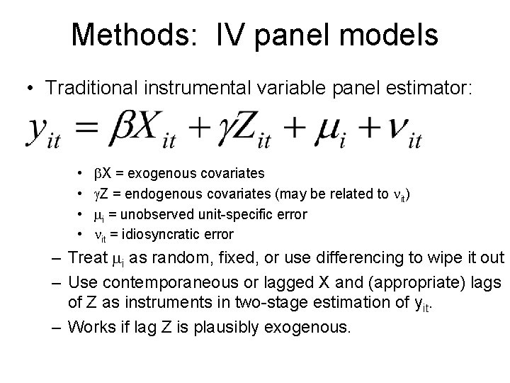
Methods: IV panel models • Traditional instrumental variable panel estimator: • • b. X = exogenous covariates g. Z = endogenous covariates (may be related to nit) mi = unobserved unit-specific error nit = idiosyncratic error – Treat mi as random, fixed, or use differencing to wipe it out – Use contemporaneous or lagged X and (appropriate) lags of Z as instruments in two-stage estimation of yit. – Works if lag Z is plausibly exogenous.

TSCS Data • Time Series Cross Section Data – Example: economic variables for industrialized countries • Often 10 -30 countries • Often ~30 -40 years of data – Beck (2001) • No specific minimum, but be suspicious of T<10 • Large N isn’t required (though not harmful)

TSCS Data: OLS PCSE • Beck & Katz 2001 – “Old” view: Use FGLS to deal with heteroskedasticity & correlated errors • Problem: This underestimates standard errors – New view: Use OLS regression • With “panel corrected” standard errors – To address panel heteroskedasticity • With FE to deal with unit heterogeneity • With lagged dependent variable in the model – To address serial correlation.

TSCS Data: Dynamics • Beck & Katz 2009 examine dynamic models – OLS PCSE with lagged Y and FE • Still appropriate • Better than some IV estimators – But, didn’t compare to System GMM. • Plumper, Troeger, Manow (2005) • FE isn’t theoretically justified and absorbs theoretically important variance • Lagged Y absorbs theoretically important temporal variation • Theory must guide model choices…

TSCS Data: Nonstationary Data • Issue: Analysis of longitudinal (time-series) data is going through big changes • Realization that strongly trending data cause problems – Random walk / unit root processes / integrated of order 1 / non -stationary data – Converse: stationary data, integrated of order zero • The “spurious regression” problem – Strategies: • Tests for “unit root” in time series & panel data • Differencing as a solution – A reason to try FD models.

Panel Data Remarks • 1. Panel data strategies are taught as “fixes” – How do I “fix” unobserved effects? – How do I “fix” dynamics/serial correlation? • But, the fixes really change what you are modeling • A FE (within) model is a very different look at your data, compared to OLS • Goal: learn the “fixes”… but get past that… start to think about interpretation • 2. Much strife in literature • People arguing over what “fix” is best • Don’t be afraid of criticism… but expect that people will weigh in with different views

Panel Data Remarks • 3. MOST IMPORTANT THING: Try a wide range of models • If your findings are robust, you’re golden • If not, differences will help you figure out what is going on… • Either way, you don’t get “surprised” when your results go away after following the suggestion of a reviewer!

Reading Discussion • Schofer, Evan and Wesley Longhofer. “The Structural Sources of Associational Life. ” Working Paper.