Pairwise sequence alignment Based on presentation by Irit

Pairwise sequence alignment Based on presentation by Irit Gat-Viks, which is based on presentation by Amir Mitchel, Introduction to bioinformatics course, Bioinformatics unit, Tel Aviv University. and of Benny shomer, Bar-Ilan university

Where we are in the course? • Ways to interrogate biobanks: – By identifier-based search (Gen. Bank etc. ) – By genome location (genome browsers) – By mining annotation files with scrips • Now: searching by sequence similarity

What is it good for? 1. Function inference – if we know something about A and A is similar to B, we can say something about B – guilt by association 2. Conservation arguments – if we know that A and B do something similar, by looking at the conserved segments we can infer which parts of A and B are important for their function 3. Looking for repeats etc. 4. Identifying the position of an m. RNA/any transcript in the genome 5. Resequencing 6. Etc.

Issues with sequence similarity • Things we’re after – A score: how well do two sequences fit? – Statistics: is this score significant or expected at random? – Regions: which parts of the query and the target sequence are actually similar/different? • Next time – How to efficiently search a large sequence database

Start from simple: Dot plots • The most intuitive method to compare two sequences. • Each dot represents a identity of two characters. • No real score/significance, but very easy to assess visually

To Reduce Random Noise in Dot Matrix • Specify a window size, w • Take w residues from each of the two sequences • Among the w pairs of residues, count how many pairs are matches • Specify a stringency

Simple Dot Matrix, Window Size 1 P V I L E P M M K V T I E M P P 1 1 V 1 I 1 L 1 E 1 P 1 1 I 1 M 1 1 1 R V 1 E 1 V 1 T 1 P 1 1

Window Size is 3 P V I L E P M M K V T I E M P P 3 1 1 1 1 V 3 1 1 I 3 1 1 L 3 1 1 1 E 1 2 1 1 1 P 1 1 1 2 1 1 1 I 1 1 1 M 1 2 1 R 1 1 V 1 1 1 E 1 1 2 1 V 1 1 2 T 1 1 1 T 1 1 2 2 1 P 1 1 1 3

Window Size is 3; Stringency is 2 P V I L E P M M K V T I E M P P 3 V 3 I 3 L 3 E 2 P 2 I M 2 R V E 2 V 2 T 2 2 P 3

Protein Sequences single residue identity 6 out of 23 identical

Insertion/Deletion, Inversion

ABCDEFGEFGHIJKLMNO tandem duplication compared to no duplication compared to self
")
What Is This? 5’ GGCGG 3’ Palindrome (Intrastrand)

Compare a sequence with itself… • Identifies low complexity/repeat regions

Dotlet example • http: //myhits. isb-sib. ch/cgi-bin/dotlet • http: //www. ncbi. nlm. nih. gov/entrez/query. f cgi? db=gene&cmd=Retrieve&dopt=full_re port&list_uids=672 • http: //www. ncbi. nlm. nih. gov/entrez/query. f cgi? db=gene&cmd=Retrieve&dopt=full_re port&list_uids=353120

Definition Alignment: A matching of two sequences. A good alignment will match many identical (similar) characters in the two sequences VLSPAD-TNVK-AWAKVGAHAAGHG ||| | | |||| VLSEAEWQ-VLHVWAKVEA--AGHG

How similar are two sequences? • The common measure of sequence similarity is their alignment score • Simpler measures, e. g. , % identity are also common • These require algorithm that compute the optimal alignment between sequences

How to present the alignment? • • | - character-wise identity : - very similar amino acids. – less similar amino acids - gap in out of the sequences

Pairwise Alignment - Scoring • The final score of the alignment is the sum of the positive scores and penalty scores: + Number of Identities + Number if Similarities - Number of Dissimilarities - Number of Gap openings - Number of Gap extensions Alignment score

Comparison methods • Global alignment – Finds the best alignment across the whole two sequences. • Local alignment – Finds regions of similarity in parts of the sequences. Global _______ __ ____ Local __ __ ____
 • Finds the alignment of")
Global Alignment • Algorithm of Needleman and Wunsch (1970) • Finds the alignment of two complete sequences: ADLGAVFALCDRYFQ |||| | ADLGRTQN-CDRYYQ • Semi-global alignment allows “free ends” GFHKKKADLGAVFALCDRYFQ |||| | ADLGRTQN-CDRYYQJKLLKJ
 • Makes an optimal alignment")
Local Alignment • Algorithm of Smith and Waterman (1981) • Makes an optimal alignment of the best segment of similarity between two sequences. ADLG |||| ADLG CDRYFQ |||| | CDRYYQ • Can return a number of well aligned segments.

Finding an optimal alignment • Pairwise alignment algorithms identify the highest scoring alignment from all possible alignments. • Different scoring systems can produce (very) different best alignments!!! • Unfortunately the number of possible alignments if pretty huge • Dynamic programming to the rescue

Intuition of Dynamic Programming • Lets say we want to align XYZ and ABC • If we already computed the optimal way to: • Align XY and AB – Opt 1 • Align XY and ABC – Opt 2 • Align XYZ and AB – Opt 3 • We now need to test three possible alignments Opt 1 Z or Opt 1 C Opt 2 Z or Opt 2 - (where “-” indicates a gap). Opt 3 C Thus, if we construct small alignments first, we are able to extend then by testing only 3 scenarios.

Formally: solving global alignment Global Alignment Problem: Input: Two sequences S=s 1…sn, T=t 1…. tm (n~m) Goal: Find an optimal alignment according to the alignment quality (or scoring). Notation: • Let (a, b) be the score (weight) of the alignment of character a with character b. • Let V(i, j) be the optimal score of the alignment of S’=s 1…si and T’=t 1…tj (0 i n, 0 j m)
 : = optimal score of the alignment of S’=s 1…si and T’=t")
V(i, j) : = optimal score of the alignment of S’=s 1…si and T’=t 1…tj (0 i n, 0 j m) V(k, l) is computed as follows: • Base conditions: Alignment with 0 elements spacing – V(i, 0) = k=0. . i (sk, -) – V(0, j) = k=0. . j (-, tk) S’=s 1. . . si-1 with T’=t 1. . . tj-1 si with tj. • Recurrence relation: V(i-1, j-1) + (si, tj) 1 i n, 1 j m: V(i, j) = max V(i-1, j) + (si, -) V(i, j-1) + (-, tj) S’=s 1. . . si with T’=t 1. . . tj-1 and ‘-’ with tj.
 for")
Optimal Alignment - Tabular Computation • Use dynamic programming to compute V(i, j) for all possible i, j values: for i=1 to n do begin For j=1 to m do begin Calculate V(i, j) using V(i-1, j-1), V(i-1, j) end Costs: match 2, mismatch/indel -1 Snapshot of computing the table
 from cell (i, j) to")
Optimal Alignment - Tabular Computation • Add back pointer(s) from cell (i, j) to father cell(s) realizing V(i, j). • Trace back the pointers from (m, n) to (0, 0) • Needleman. Wunsch, ‘ 70 Backtracking the alignment
. • V(i, j) :")
Solving Local Alignment • Algorithm of Smith and Waterman (1981). • V(i, j) : the value of optimal local alignment between S[1. . i] and T[1. . j] • Assume the weights fulfill the following condition: (x, y) = 0 if x, y match 0 o/w (mismatch or indel)
 A scheme of the algorithm: • Find maximum similarity between")
Computing Local Alignment (2) A scheme of the algorithm: • Find maximum similarity between suffixes of S’=s 1. . . si and T’=t 1. . . tj • Discard the prefixes S’=s 1. . . si, and T’=t 1. . . tj whose similarity is 0 (and therefore decrease the overall similarity) • Find the indices i*, j* of S and T respectively after which the similarity only decreases. Algorithm - Recursive Definition Base Condition: i, j V(i, 0) = 0, V(0, j) = 0 Recursion Step: i>0, j>0 0, V(i, j) = max V(i-1, j-1) + (si, tj), V(i, j-1) + (-, tj), V(i-1, j) + (si, -) Compute i*, j* s. t. V(i*, j*) = max 1 i n, 1 j m. V(i, j)

• As usual the pointers are created while filling the values in the table, • The alignments are found by tracking the pointers from cell (i*, j*) until reaching an entry (i’, j’) that has value 0.
 operations for both global and")
Computational complexity • Computing the table requires O(n 2) operations for both global and local alignment • Saving the pointers for traceback - O(n 2) • But – what if we are only interested in the optimal alignment score? • Only need to remember the last row – O(n) space

Outline • We now figured out • What an alignment is • What alignment score consists of • How to ± efficiently compute an optimal alignment • Still left to figure out • Where do we obtain good σ(i, j) values • When do we use global/local alignment • How to use alignment to search large databases

Scoring amino acid similarity • Identity: Count the number of identical matches, divide by length of aligned region. The homology rule: above 25% for amino acids, above 75% for nucleotides. • Similarity: A less well defined measure Category Amino Acids and Amides Asp (D) Glu(E) Asn (N) Gln (Q) Basic His (H) Lys (K) Arg (R) Aromatic Phe (F) Tyr (Y) Trp (W) Hydrophilic Ala (A) Cys (C) Gly (G) Pro (P) Ser (S) Thr (T) Hydrophobic Ile (I) Leu (L) Met (M) Val (V) • A problematic idea: Give positive score for aligning amino acids from the same group Can we find a better definition for similarity?

Scoring System based on evolution • Some substitutions are more frequent than other substitutions • Chemically similar amino acids can be replaced without severely effecting the protein’s function and structure • Orthologous proteins: proteins derived from the same common ancestor • By comparing reasonably close orthologous proteins we can compute the relative frequencies of different amino acid changes • Amino acid substitution matrices: Families of matrices that list the probability of change from one amino acid to another during evolution (i. e. , defining identity and similarity relationships between amino acids). • The two most popular matrices are the PAM and the BLOSUM matrix

PAM matrix • PAM units measure evolutionary distance. • 1 PAM unit indicates the probability of 1 point mutation per 100 residues. • Multiplying PAM 1 by itself gives higher PAMs matrices that are suitable for larger evolutionary distance. • JTT matrices are a newer generation of PAMs

PAM 1

PAM 250

Log Odds matrices • The score might arise from bias in amino acid frequency -> We use the log odds of the PAM matrix. (120 PAM)

Rules of thumb • The most widely used PAM 250 is good for about 20% identity between the proteins • 40% --> PAM 120 • 50% --> PAM 80 • 60% --> PAM 60

PAM vs. BLUSOM • Choosing n – Different BLOSUM matrices are derived from blocks with different identity percentage. (e. g. , blosum 62 is derived from an alignment of sequences that share at least 62% identity. ) Larger n smaller evolutionary distance. – Single PAM was constructed from at least 85% identity dataset. Different PAM matrices were computationally derived from it. Larger n larger evolutionary distance Observed % Difference 1 10 20 30 40 50 60 70 80 Evolutionary distance (PAM) 1 11 23 38 56 80 120 159 250 BLOSUM 99 90 80 70 60 50 40 30 20 62 • Blosum matrices are newer (based on more sequences)

Gap parameters • Observation: Alignments can differ significantly when using different gap parameters. • Assumption: For each matrix there are constant default parameters that produce optimum alignments. • Each matrix was checked with different parameters until a “true” alignment was reached. – Where can we obtain “true” alignments? – We can use sequence alignments based on structural alignments. – The structural alignments are “true” for our purpose.

DNA scoring matrices • Uniform substitutions in all nucleotides: From To A G 2 -6 2 C T -6 -6 Mismatch C T 2 -6 2 Match
")
DNA scoring matrices • The bases are divided to two groups, purines (A, G) and pyrmidines (C, T) • Mutations are divided into transitions and transversions. • Transitions – purine to purine or pyrmidine to pyrmidine (4 possibilities). • Transversions – purine to pyrmidine or pyrmidine to purine. (8 possibilities). • By chance alone transversions should occur twice than transition. • De-facto transitions are more frequent than transversions • Bottom line: Meaningful DNA substitution matrices can be defined

DNA scoring matrices • Non-uniform substitutions in all nucleotides: From To A G 2 -4 2 C T -6 -6 Mismatch transversion transition C T 2 -4 2 Match

Evaluation • Remember that one of our goals was to estimate significance of the scores • How can we estimate the significance of the alignment? • Which alignment is better ? A T C G C A T - G C ? A A C A A - A A Does the score arise from order or from composition ?

Evaluation - bootstrap approach • Data with same composition but different order: 1. Shuffle one of the sequences. 2. Re-align and score. 3. Repeat numerous times. 4. Calculate the mean and standard deviation of shuffled alignments scores.

Evaluation - bootstrap approach • Data with the same composition but with a different order: Shuffle one of the sequences Align with the second sequence Calculate mean and standard deviation of shuffled alignments Compare alignment score with mean of shuffled alignments

Evaluation • We can compare the score of the original alignment with the average score of the shuffled alignments. • Thumb rule: If: original alignment >>average score + 6*SD Then: the alignment is statistically significant.

Global or local? • Two human transcription factors: 1. SP 1 factor, binds to GC rich areas. 2. EGR-1 factor, active at differentiation stage (Fasta fromats from http: //us. expasy. org/sprot/)
. MSDQDHSMDEMTAVVKIEKGVGGNNGGNGNGGGAFSQARSSSTGSSSSTGGGGQESQPSP LALLAATCSRIESPNENSNNSQGPSQSGGTGELDLTATQLSQGANGWQIISSSSGATPTS KEQSGSSTNGSNGSESSKNRTVSGGQYVVAAAPNLQNQQVLTGLPGVMPNIQYQVIPQFQ")
>sp|P 08047|SP 1_HUMAN Transcription factor Sp 1 - Homo sapiens (Human). MSDQDHSMDEMTAVVKIEKGVGGNNGGNGNGGGAFSQARSSSTGSSSSTGGGGQESQPSP LALLAATCSRIESPNENSNNSQGPSQSGGTGELDLTATQLSQGANGWQIISSSSGATPTS KEQSGSSTNGSNGSESSKNRTVSGGQYVVAAAPNLQNQQVLTGLPGVMPNIQYQVIPQFQ TVDGQQLQFAATGAQVQQDGSGQIQIIPGANQQIITNRGSGGNIIAAMPNLLQQAVPLQG LANNVLSGQTQYVTNVPVALNGNITLLPVNSVSAATLTPSSQAVTISSSGSQESGSQPVT SGTTISSASLVSSQASSSSFFTNANSYSTTTTTSNMGIMNFTTSGSSGTNSQGQTPQRVS GLQGSDALNIQQNQTSGGSLQAGQQKEGEQNQQTQQQQILIQPQLVQGGQALQALQAAPL SGQTFTTQAISQETLQNLQLQAVPNSGPIIIRTPTVGPNGQVSWQTLQLQNLQVQNPQAQ TITLAPMQGVSLGQTSSSNTTLTPIASAASIPAGTVTVNAAQLSSMPGLQTINLSALGTS GIQVHPIQGLPLAIANAPGDHGAQLGLHGAGGDGIHDDTAGGEEGENSPDAQPQAGRRTR REACTCPYCKDSEGRGSGDPGKKKQHICHIQGCGKVYGKTSHLRAHLRWHTGERPFMCTW SYCGKRFTRSDELQRHKRTHTGEKKFACPECPKRFMRSDHLSKHIKTHQNKKGGPGVALS VGTLPLDSGAGSEGSGTATPSALITTNMVAMEAICPEGIARLANSGINVMQVADLQSINI SGNGF >sp|P 18146|EGR 1_HUMAN Early growth response protein 1 (EGR-1) (Krox-24 protein) (ZIF 268) (Nerve growth factorinduced protein A) (NGFI-A) (Transcription factor ETR 103) (Zinc finger protein 225) (AT 225) - Homo sapiens (Human). MAAAKAEMQLMSPLQISDPFGSFPHSPTMDNYPKLEEMMLLSNGAPQFLGAAGAPEGSGS NSSSSSSGGGGGSNSSSSSSTFNPQADTGEQPYEHLTAESFPDISLNNEKVLVETS YPSQTTRLPPITYTGRFSLEPAPNSGNTLWPEPLFSLVSGLVSMTNPPASSSSAPSPAAS SASASQSPPLSCAVPSNDSSPIYSAAPTFPTPNTDIFPEPQSQAFPGSAGTALQYPPPAY PAAKGGFQVPMIPDYLFPQQQGDLGLGTPDQKPFQGLESRTQQPSLTPLSTIKAFATQSG SQDLKALNTSYQSQLIKPSRMRKYPNRPSKTPPHERPYACPVESCDRRFSRSDELTRHIR IHTGQKPFQCRICMRNFSRSDHLTTHIRTHTGEKPFACDICGRKFARSDERKRHTKIHLR QKDKKADKSVVASSATSSLSSYPSPVATSYPSPVTTSYPSPATTSYPSPVPTSFSSPGSS TYPSPVHSGFPSPSVATTYSSVPPAFPAQVSSFPSSAVTNSFSASTGLSDMTATFSPRTI EIC

SP 1 at swissprot

EGR 1 at swissprot

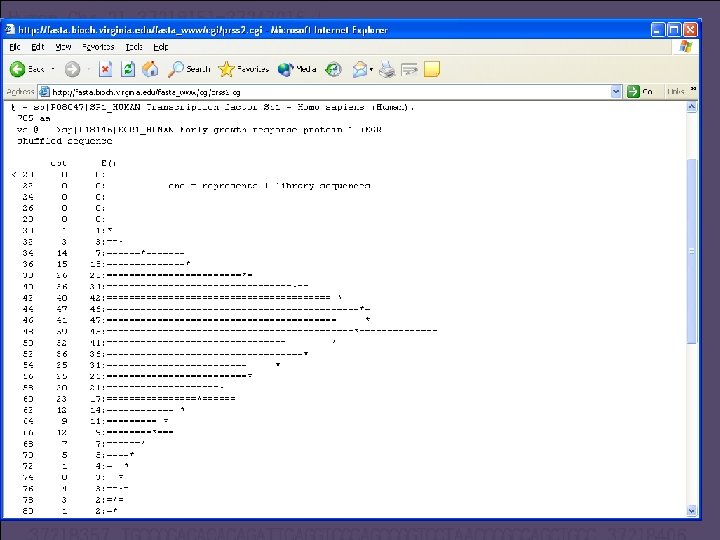
Available softwares… • http: //en. wikipedia. org/wiki/Sequence_alignment_software • http: //fasta. bioch. virginia. edu/fasta_www/home. html – LAlign (local alignment), PLalign(dot plot) – PRSS/ PRFX (significance by Monte Carlo) • http: //bioportal. weizmann. ac. il/toolbox/overview. html (Many useful software), Needle, Water. • Bl 2 seq (NCBI)

Using LAlign • http: //www. ch. embnet. org/software/LALIG N_form. html • http: //www. ncbi. nlm. nih. gov/entrez/viewer. f cgi? val=NP_006758. 2 • http: //www. ncbi. nlm. nih. gov/entrez/viewer. f cgi? val=NP_066300. 1

Bl 2 Seq at NCBI http: //www. ncbi. nlm. nih. gov/blast/bl 2 seq/wblast 2. cgi

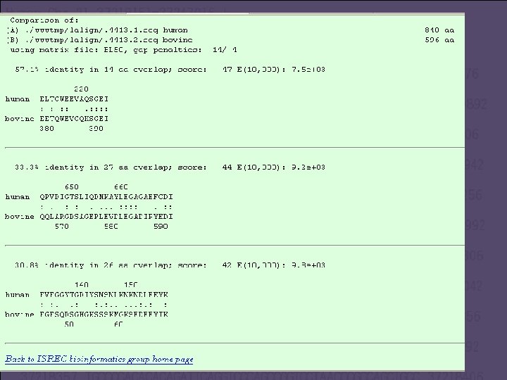
Bl 2 seq results

Conclusions • The proteins share only a limited area of sequence similarity. Therefore, the use of local alignment is recommended. • We found a local alignment that pointed to a possible structural similarity, which points to a possible function similarity. • Reasons to make Global alignment: • Checking minor differences between close homologous. • Analyzing polymorphism. • A good reason

Sequence comparisons Goal: Comparing two specific sequences Goal: similarity search on sequence database Single pairwise comparisons Multiple pairwise comparisons We wish to optimize for accuracy, not speed We wish to optimize for speed, not accuracy Dynamic programming methods (Smith-Waterman, Needleman -Wunsch) BLAST, FASTA programs Identify homologous, common domains, common active sites etc. Next goal: refine database search, are the reported matches really interesting?
- Slides: 61