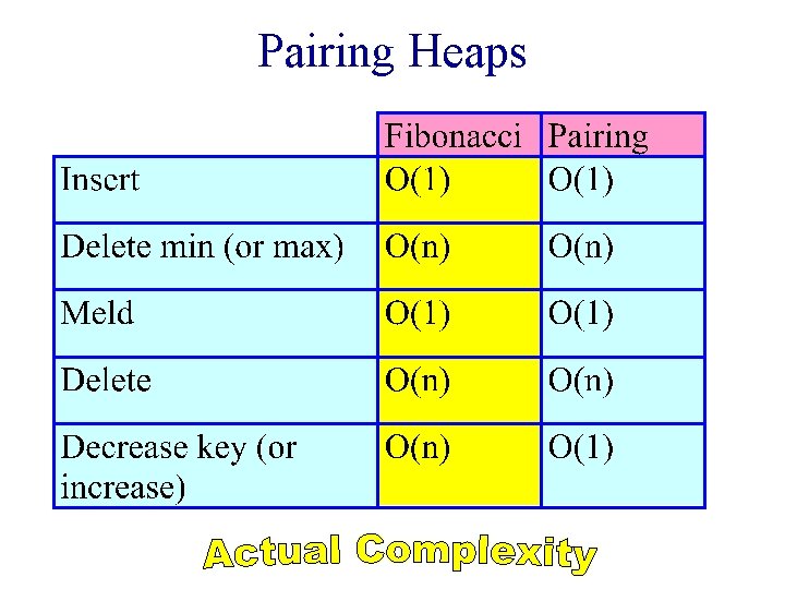
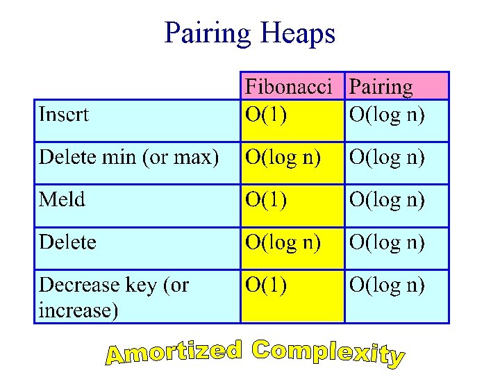
Pairing Heaps Pairing Heaps Pairing Heaps Experimental results

Pairing Heaps

Pairing Heaps

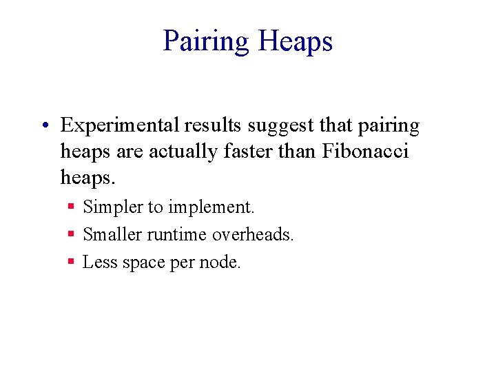
Pairing Heaps • Experimental results suggest that pairing heaps are actually faster than Fibonacci heaps. § Simpler to implement. § Smaller runtime overheads. § Less space per node.

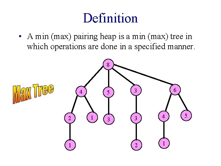
Definition • A min (max) pairing heap is a min (max) tree in which operations are done in a specified manner. 8 4 2 1 1 6 5 3 3 3 4 2 1 5

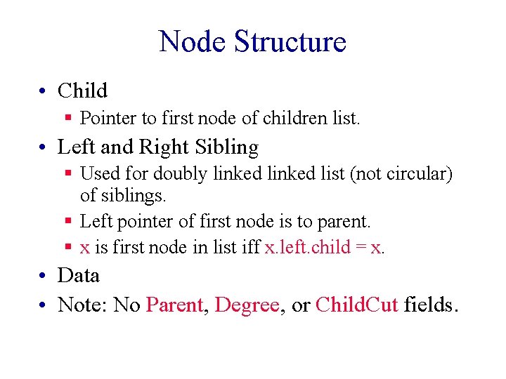
Node Structure • Child § Pointer to first node of children list. • Left and Right Sibling § Used for doubly linked list (not circular) of siblings. § Left pointer of first node is to parent. § x is first node in list iff x. left. child = x. • Data • Note: No Parent, Degree, or Child. Cut fields.

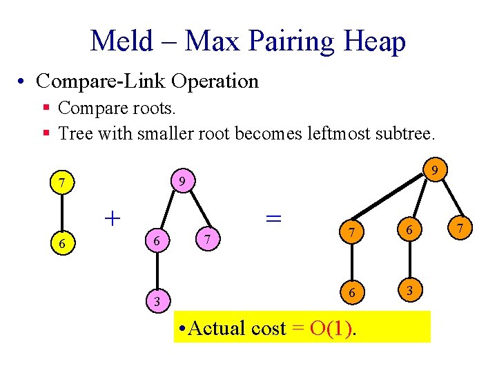
Meld – Max Pairing Heap • Compare-Link Operation § Compare roots. § Tree with smaller root becomes leftmost subtree. 9 7 + 6 9 6 3 7 = 7 6 6 3 • Actual cost = O(1). 7

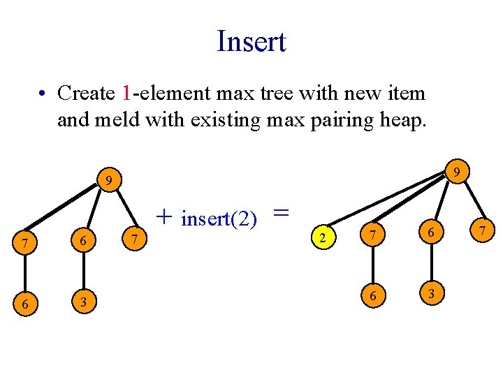
Insert • Create 1 -element max tree with new item and meld with existing max pairing heap. 9 9 7 6 6 3 7 + insert(2) = 2 7 6 6 3 7

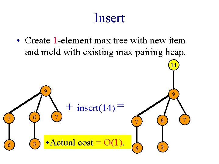
Insert • Create 1 -element max tree with new item and meld with existing max pairing heap. 14 9 7 6 6 3 9 7 + insert(14) = • Actual cost = O(1). 7 6 6 3 7

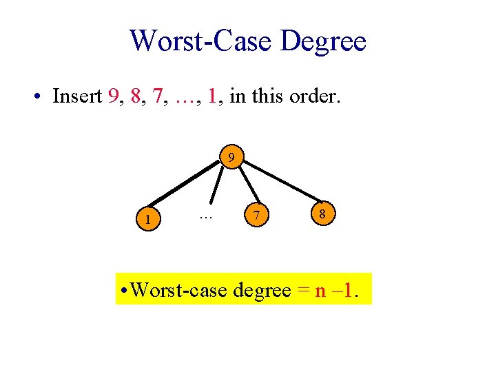
Worst-Case Degree • Insert 9, 8, 7, …, 1, in this order. 9 1 … 7 8 • Worst-case degree = n – 1.

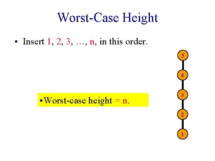
Worst-Case Height • Insert 1, 2, 3, …, n, in this order. 5 4 • Worst-case height = n. 3 2 1

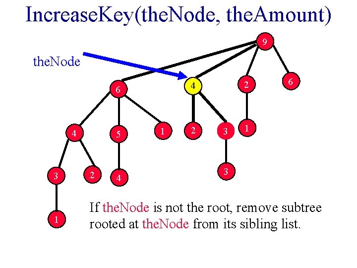
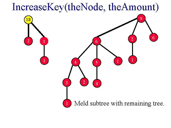
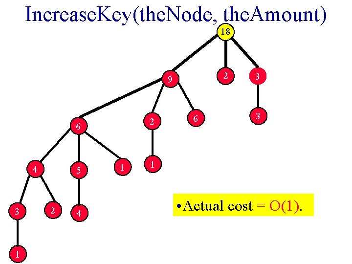
Increase. Key(the. Node, the. Amount) • Since nodes do not have parent fields, we cannot easily check whether the key in the. Node becomes larger than that in its parent. • So, detach the. Node from sibling doublylinked list and meld.

Increase. Key(the. Node, the. Amount) 9 the. Node 6 4 5 2 4 1 2 3 6 1 3 3 2 1 If the. Node is not the root, remove subtree rooted at the. Node from its sibling list. 4

Increase. Key(the. Node, the. Amount) 9 18 2 3 2 6 3 4 3 1 5 2 1 6 1 4 Meld subtree with remaining tree.

Increase. Key(the. Node, the. Amount) 18 2 9 2 6 4 3 1 5 2 4 1 6 3 3 1 • Actual cost = O(1).

Delete Max • If empty => fail. • Otherwise, remove tree root and meld subtrees into a single max tree. • How to meld subtrees? § Good way => O(log n) amortized complexity for remove max. § Bad way => O(n) amortized complexity.

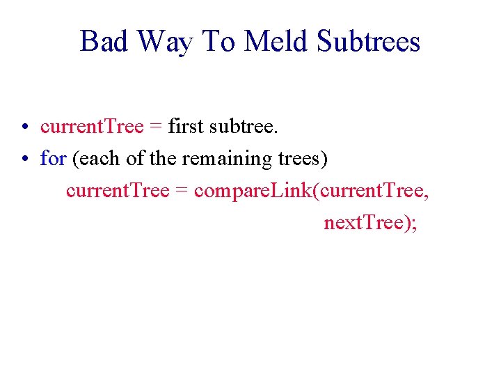
Bad Way To Meld Subtrees • current. Tree = first subtree. • for (each of the remaining trees) current. Tree = compare. Link(current. Tree, next. Tree);

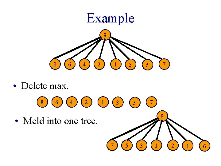
Example 9 8 6 4 2 1 3 7 5 • Delete max. 8 6 4 2 1 3 7 5 8 • Meld into one tree. 7 5 3 1 2 4 6

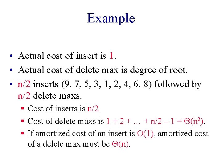
Example • Actual cost of insert is 1. • Actual cost of delete max is degree of root. • n/2 inserts (9, 7, 5, 3, 1, 2, 4, 6, 8) followed by n/2 delete maxs. § Cost of inserts is n/2. § Cost of delete maxs is 1 + 2 + … + n/2 – 1 = Q(n 2). § If amortized cost of an insert is O(1), amortized cost of a delete max must be Q(n).

Good Ways To Meld Subtrees • • Two-pass scheme. Multipass scheme. Both have same asymptotic complexity. Two-pass scheme gives better observed performance.

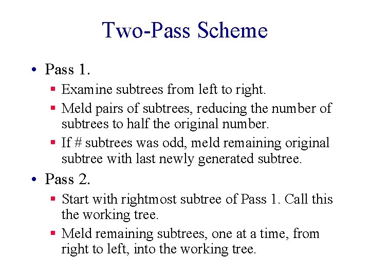
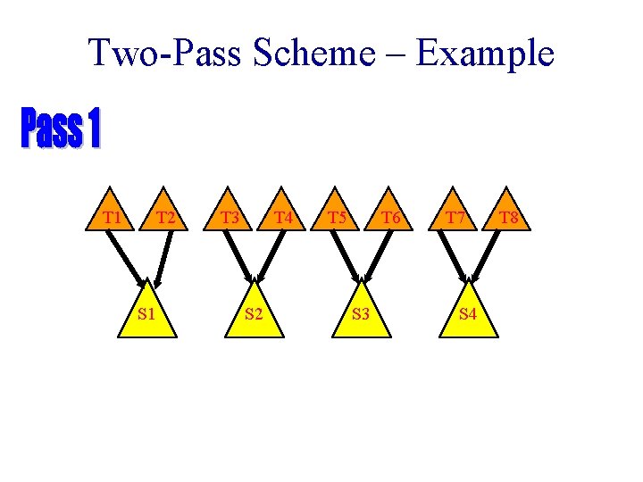
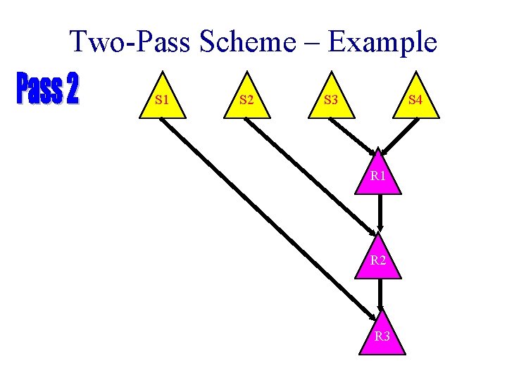
Two-Pass Scheme • Pass 1. § Examine subtrees from left to right. § Meld pairs of subtrees, reducing the number of subtrees to half the original number. § If # subtrees was odd, meld remaining original subtree with last newly generated subtree. • Pass 2. § Start with rightmost subtree of Pass 1. Call this the working tree. § Meld remaining subtrees, one at a time, from right to left, into the working tree.

Two-Pass Scheme – Example T 1 T 2 S 1 T 3 T 4 S 2 T 5 T 6 S 3 T 7 S 4 T 8

Two-Pass Scheme – Example S 1 S 2 S 3 S 4 R 1 R 2 R 3

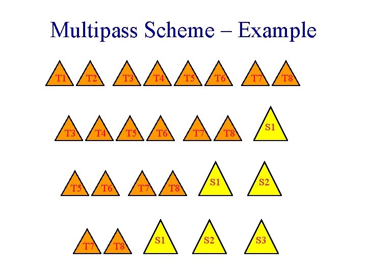
Multipass Scheme • Place the subtrees into a FIFO queue. • Repeat until 1 tree remains. § Remove 2 subtrees from the queue. § Meld them. § Put the resulting tree onto the queue.

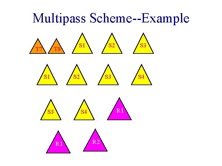
Multipass Scheme – Example T 1 T 2 T 3 T 4 T 5 T 6 T 7 T 4 T 6 T 7 T 8 T 5 T 7 T 8 S 1 T 6 T 8 S 1 S 2 T 7 T 8 S 1 S 2 S 3

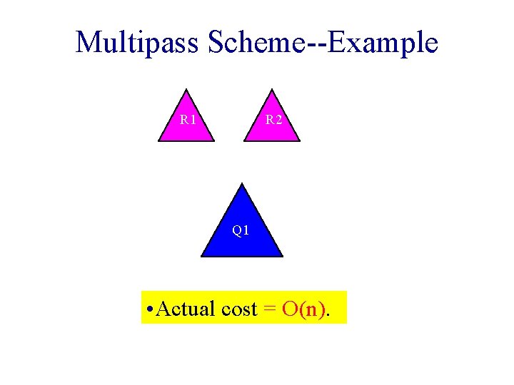
Multipass Scheme--Example T 7 T 8 S 1 S 2 S 3 S 4 R 1 S 3 R 2

Multipass Scheme--Example R 1 R 2 Q 1 • Actual cost = O(n).

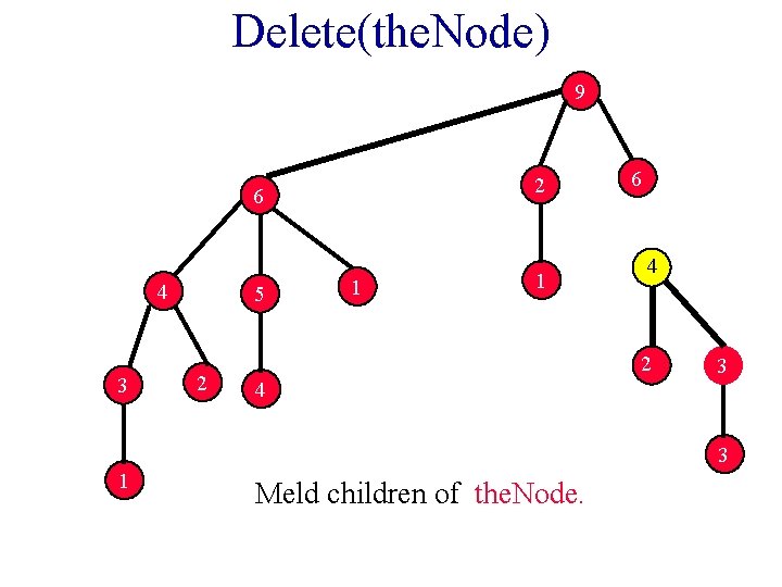
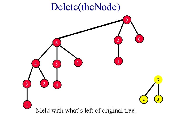
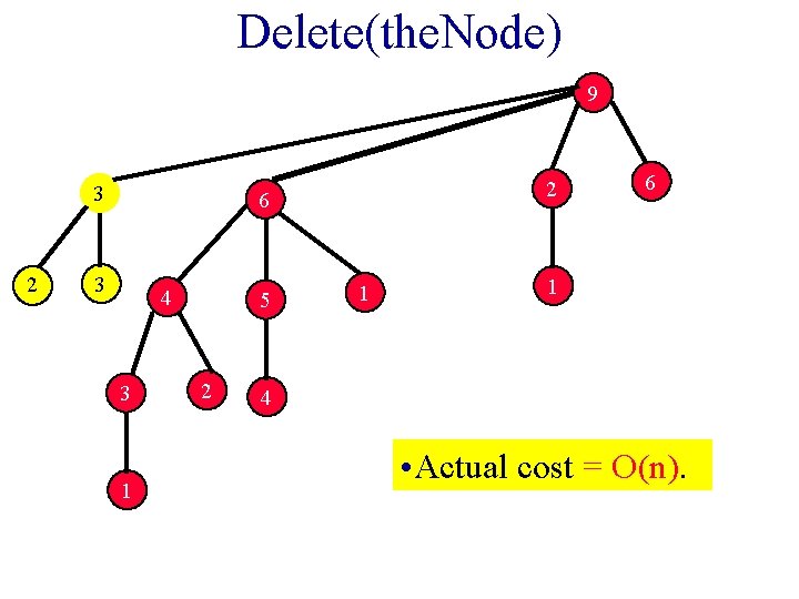
Delete Nonroot Element • Remove the. Node from its sibling list. • Meld children of the. Node using either 2 -pass or multipass scheme. • Meld resulting tree with what’s left of original tree.

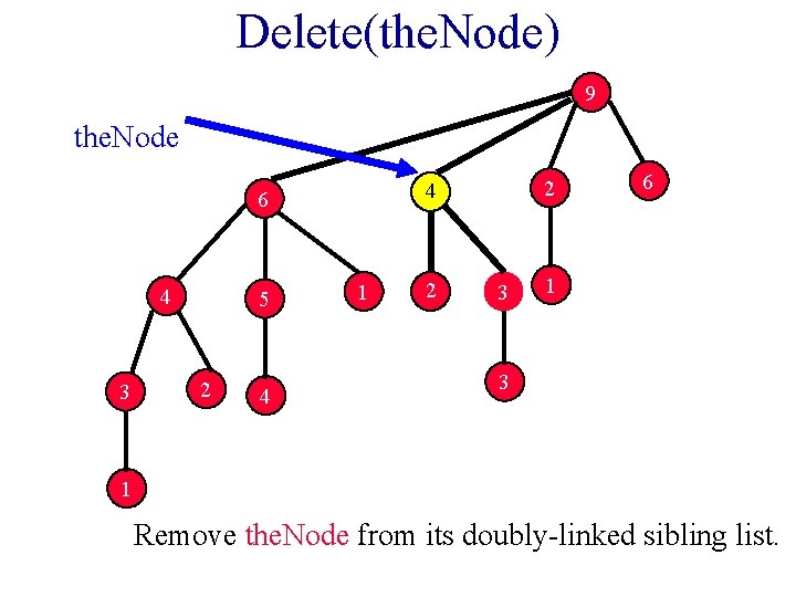
Delete(the. Node) 9 the. Node 6 4 3 5 2 4 1 2 3 6 1 3 1 Remove the. Node from its doubly-linked sibling list.

Delete(the. Node) 9 2 6 4 3 5 2 1 1 6 4 2 4 3 3 1 Meld children of the. Node.

Delete(the. Node) 9 2 6 4 3 5 2 1 6 1 3 4 2 1 Meld with what’s left of original tree. 3

Delete(the. Node) 9 3 2 2 6 3 4 3 1 5 2 1 6 1 4 • Actual cost = O(n).