p h Slides from Yann Chemla blame him

p = h/λ Slides from Yann Chemla— blame him if anything is wrong!

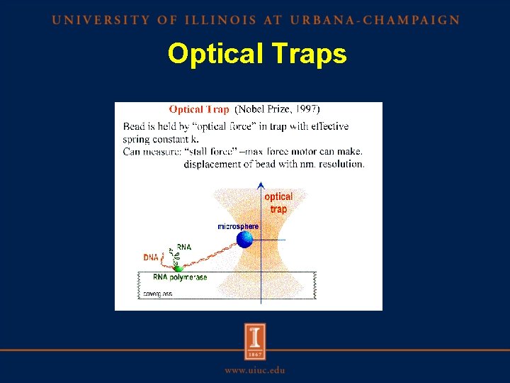
Optical Traps

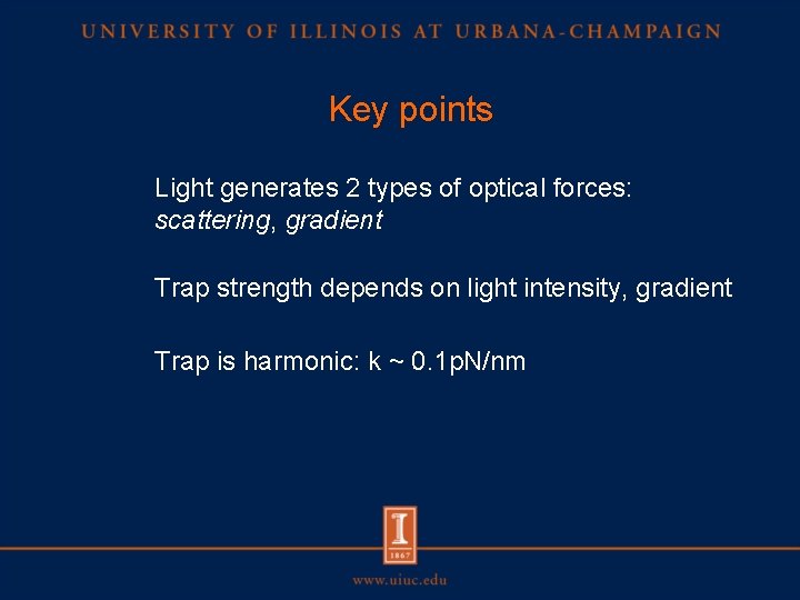
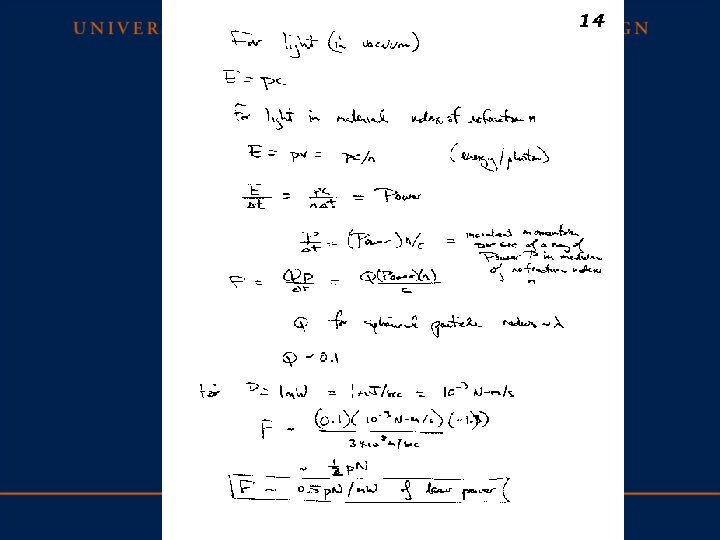
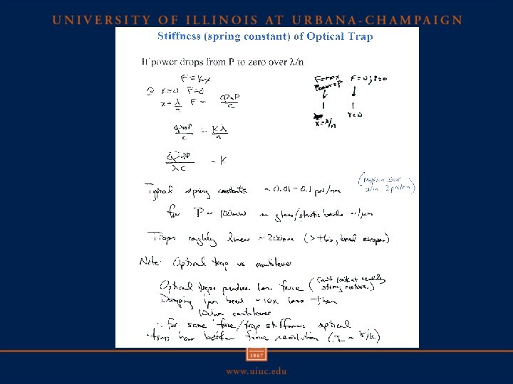
Key points Light generates 2 types of optical forces: scattering, gradient Trap strength depends on light intensity, gradient Trap is harmonic: k ~ 0. 1 p. N/nm

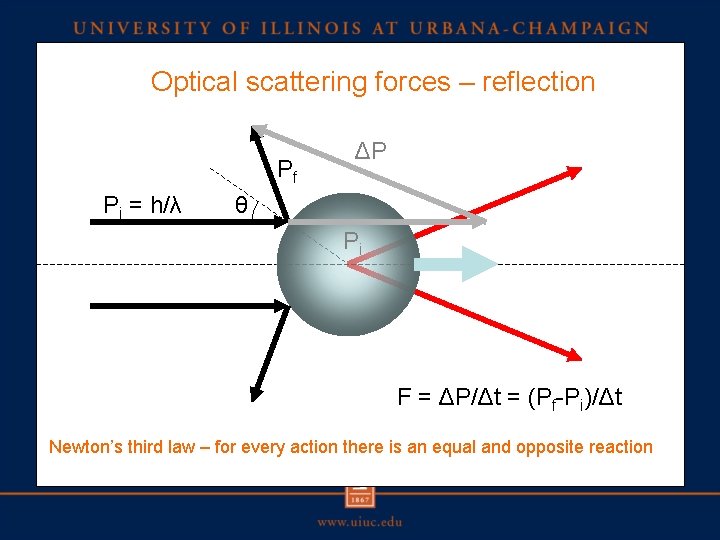
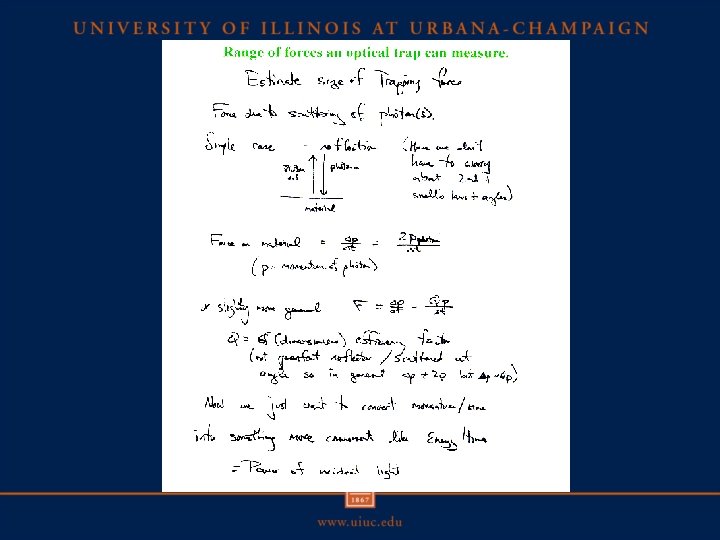
Optical scattering forces – reflection Pf Pi = h/λ ΔP θ Pi F = ΔP/Δt = (Pf-Pi)/Δt Newton’s third law – for every action there is an equal and opposite reaction

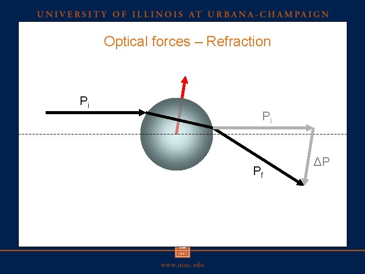
Optical forces – Refraction Pi Pi Pf ΔP

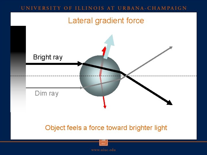
Lateral gradient force Bright ray Dim ray Object feels a force toward brighter light

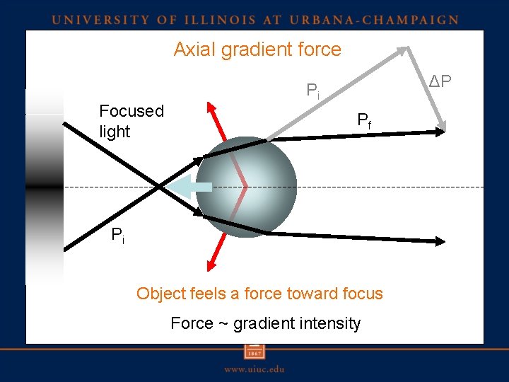
Axial gradient force Focused light ΔP Pi Pf Pi Object feels a force toward focus Force ~ gradient intensity

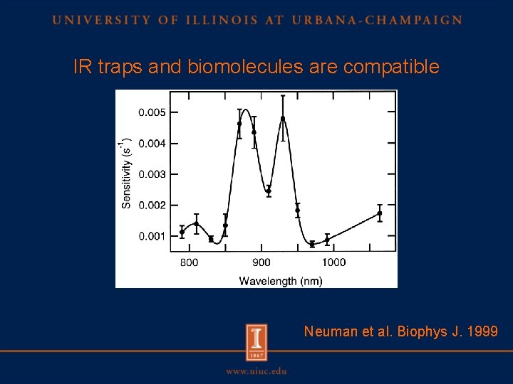
IR traps and biomolecules are compatible Neuman et al. Biophys J. 1999

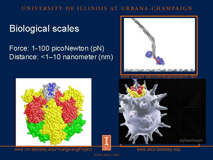
Biological scales Force: 1 -100 pico. Newton (p. N) Distance: <1– 10 nanometer (nm) www. scripps. edu/cb/milligan/projects. html www. cnr. berkeley. edu/~hongwang/Project www. alice. berkeley. edu

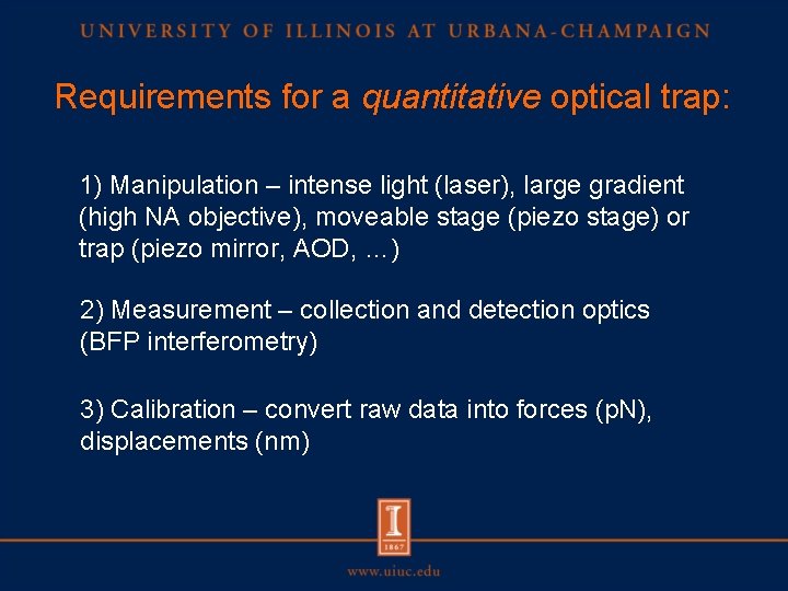
Requirements for a quantitative optical trap: 1) Manipulation – intense light (laser), large gradient (high NA objective), moveable stage (piezo stage) or trap (piezo mirror, AOD, …) 2) Measurement – collection and detection optics (BFP interferometry) 3) Calibration – convert raw data into forces (p. N), displacements (nm)

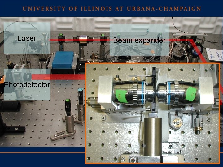
Laser Beam expander Photodetector Condenser Objective

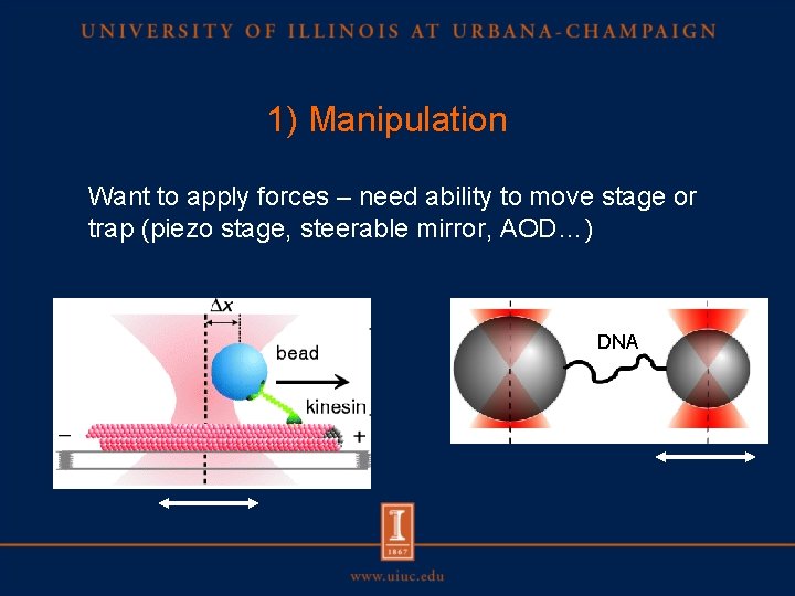
1) Manipulation Want to apply forces – need ability to move stage or trap (piezo stage, steerable mirror, AOD…) DNA

2) Measurement Want to measure forces, displacements – need to detect deflection of bead from trap center 1) Video microscopy 2) Laser-based method – Back-focal plane interferometry

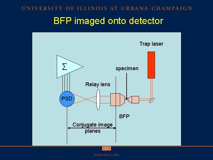
BFP imaged onto detector Trap laser ∑ specimen Relay lens PSD BFP Conjugate image planes

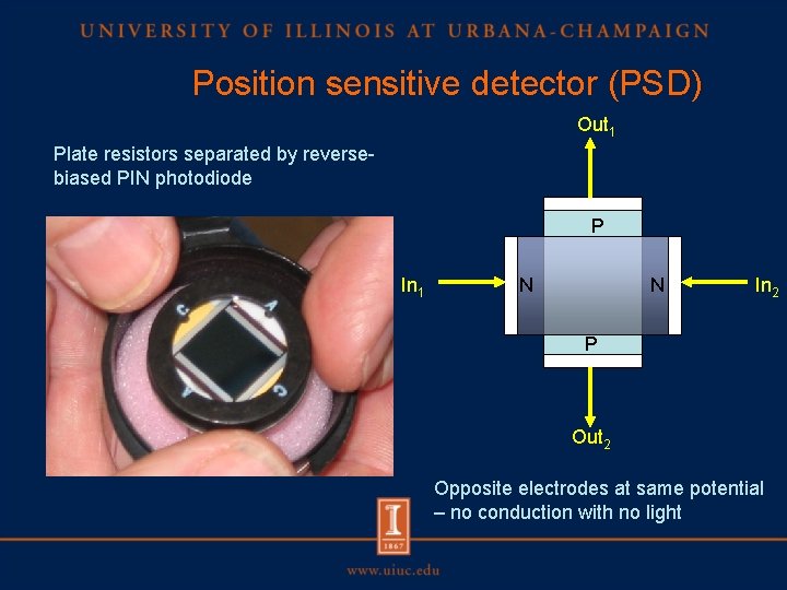
Position sensitive detector (PSD) Out 1 Plate resistors separated by reversebiased PIN photodiode P In 1 N N In 2 P Out 2 Opposite electrodes at same potential – no conduction with no light

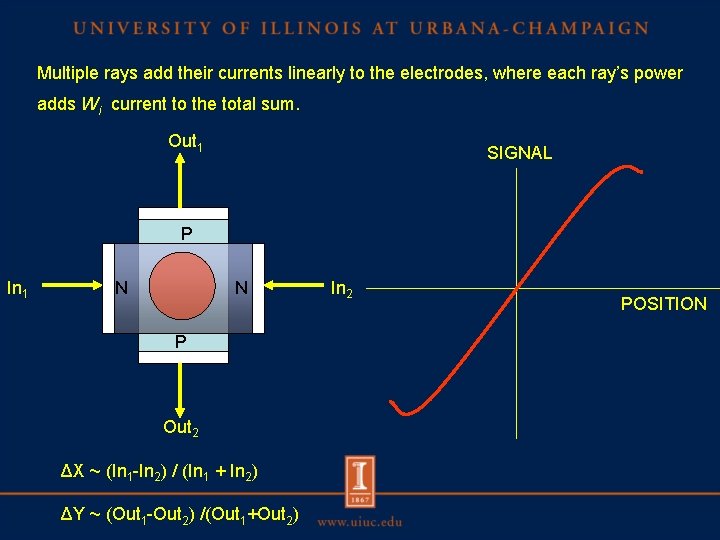
Multiple rays add their currents linearly to the electrodes, where each ray’s power adds Wi current to the total sum. Out 1 SIGNAL P In 1 N N P Out 2 ΔX ~ (In 1 -In 2) / (In 1 + In 2) ΔY ~ (Out 1 -Out 2) /(Out 1+Out 2) In 2 POSITION

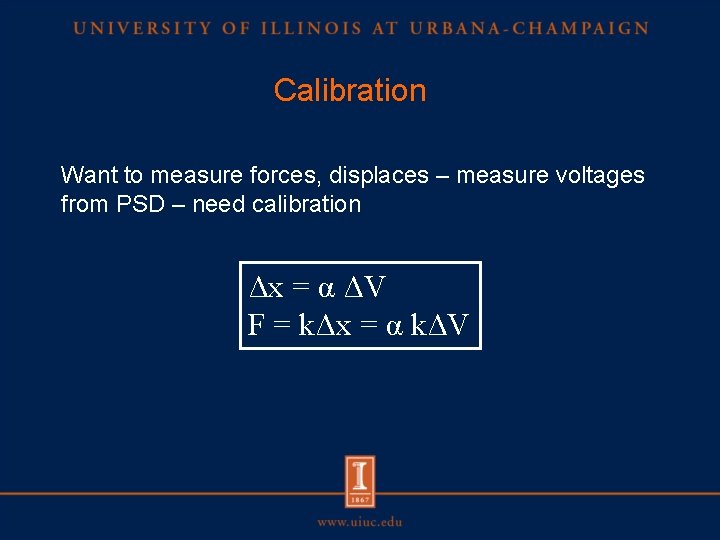
Calibration Want to measure forces, displaces – measure voltages from PSD – need calibration Δx = α ΔV F = kΔx = α kΔV

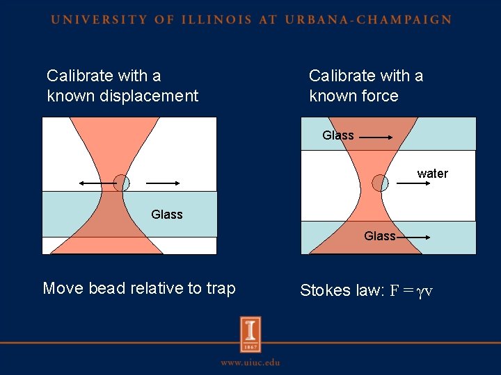
Calibrate with a known displacement Calibrate with a known force Glass water Glass Move bead relative to trap Stokes law: F = γv

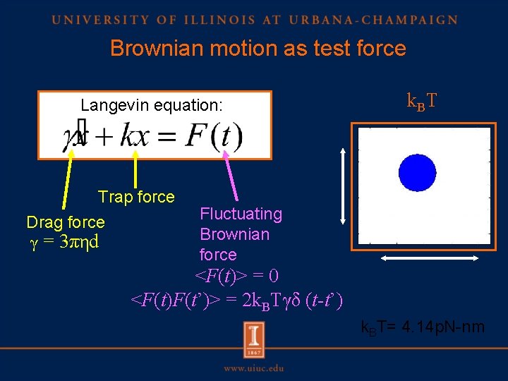
Brownian motion as test force Langevin equation: Trap force Drag force γ = 3πηd k. BT Fluctuating Brownian force <F(t)> = 0 <F(t)F(t’)> = 2 k. BTγδ (t-t’) k. BT= 4. 14 p. N-nm

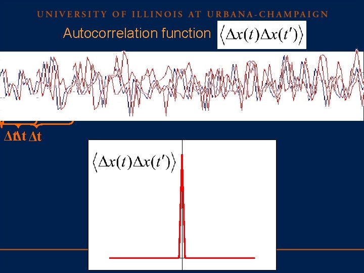
Autocorrelation function ΔtΔt Δt

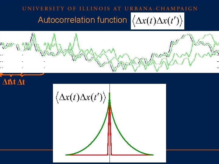
Autocorrelation function ΔtΔt Δt

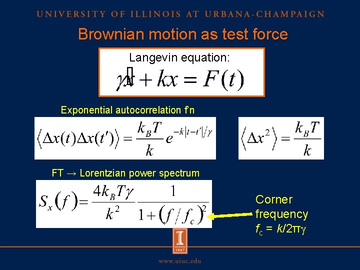
Brownian motion as test force Langevin equation: Exponential autocorrelation f’n FT → Lorentzian power spectrum Corner frequency fc = k/2πg

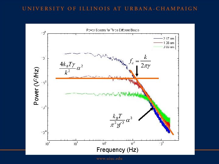
Power (V 2/Hz) Frequency (Hz)

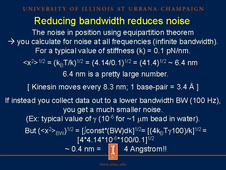
Reducing bandwidth reduces noise. The noise in position using equipartition theorem you calculate for noise at all frequencies (infinite bandwidth). For a typical value of stiffness (k) = 0. 1 p. N/nm. <x 2>1/2 = (k. BT/k)1/2 = (4. 14/0. 1)1/2 = (41. 4)1/2 ~ 6. 4 nm is a pretty large number. [ Kinesin moves every 8. 3 nm; 1 base-pair = 3. 4 Å ] If instead you collect data out to a lower bandwidth BW (100 Hz), you get a much smaller noise. (Ex: typical value of g (10 -6 for ~1 mm bead in water). But (<x 2>BW)1/2 = [∫const*(BW)dk]1/2= [(4 k. BTg 100)/k]1/2 = [4*4. 14*10 -6*100/0. 1]1/2 ~ 0. 4 nm = 4 Angstrom!!

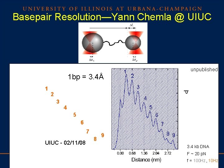
Basepair Resolution—Yann Chemla @ UIUC 1 bp = 3. 4Å 1 1 unpublished 2 3 4 5 6 6 7 7 UIUC - 02/11/08 8 9 3. 4 kb DNA F ~ 20 p. N f = 100 Hz, 10 Hz

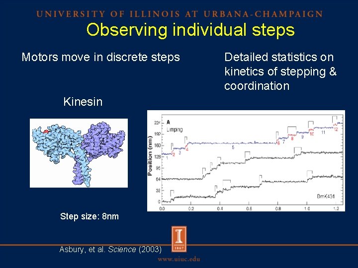
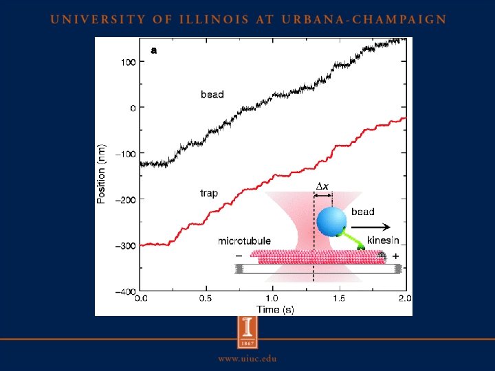
Observing individual steps Motors move in discrete steps Kinesin Step size: 8 nm Asbury, et al. Science (2003) Detailed statistics on kinetics of stepping & coordination

Class evaluation 1. What was the most interesting thing you learned in class today? 2. What are you confused about? 3. Related to today’s subject, what would you like to know more about? 4. Any helpful comments. Answer, and turn in at the end of class.