P 2 P Networks Unstructured Networks Pedro Garca

P 2 P Networks Unstructured Networks Pedro García López Universitat Rovira I Virgili Pedro. garcia@urv. net

Index 1. 2. 3. 4. 5. 6. Introduction Centralized Model: Napster Decentralized Model: Gnutella Small World: Freenet Hybrid Model: Morpheus Data location in unstructured networks

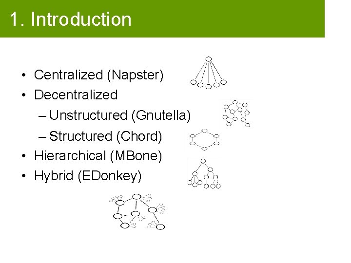
1. Introduction • Centralized (Napster) • Decentralized – Unstructured (Gnutella) – Structured (Chord) • Hierarchical (MBone) • Hybrid (EDonkey)

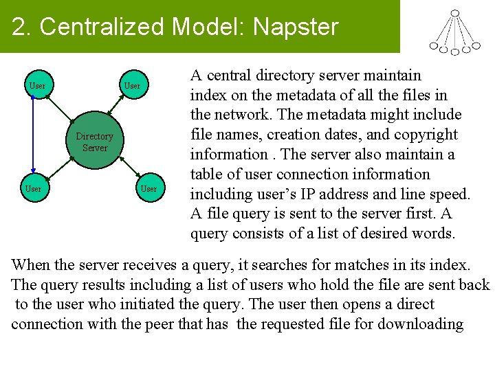
2. Centralized Model: Napster User Directory Server User A central directory server maintain index on the metadata of all the files in the network. The metadata might include file names, creation dates, and copyright information. The server also maintain a table of user connection information including user’s IP address and line speed. A file query is sent to the server first. A query consists of a list of desired words. When the server receives a query, it searches for matches in its index. The query results including a list of users who hold the file are sent back to the user who initiated the query. The user then opens a direct connection with the peer that has the requested file for downloading

List of (technical) issues with Napster • Many clients just aren’t accessible – Firewalls can limit incoming connections to clients – Many client systems come and go (churn) – Round trip times to Nepal are slow… – Slow “upload” speeds are common connections • Clients might withdraw a file unexpectedly – E. g. if low on disk space, or if they download something on top of a song they aren’t listening to anymore

More (technical) issues with Napster • Industry has been attacking the service… and not just in court of law – Denial of service assaults on core servers – Some clients lie about content (e. g. serve Frank Sinatra in response to download for Eminem) – Hacking Napster “clients” to run the protocol in various broken (disruptive) ways – And trying to figure out who is serving which files, in order to sue those people

What problems are “fundamental”? • If we assume clients serve up the same stuff people download, the number of sources for a less popular item will be very small • Under assumption that churn is a constant, these less popular items will generally not be accessible. • But experiments show that clients fall into two categories: – Well-connected clients that hang around – Poorly-connected clients that also churn – … this confuses the question

What problems are fundamental? • One can have, some claim, as many electronic personas as one has the time and energy to create. – Judith S. Donath. • So-called “Sybil attack…. ” • Attacker buys a high performance computer cluster • It registers many times with Napster using a variety of IP addresses (maybe 10’s of thousands of times) • Thinking these are real, Napster lists them in download pages. Real clients get poor service or even get snared • Studies show that no p 2 p system can easily defend against Sybil attacks!

Refined Napster structure • Early Napster just listed anything. Later: – Enhanced directory servers to probe clients, track their health. Uses an automated reporting of download problems to trim “bad sources” from list – [Incentives] Ranks data sources to preferentially list clients who… • Have been up for a long time, and • Seem to have fast connections, and • Appear to be “close” to the client doing the download (uses notion of “Internet distance”) – Implement parallel downloads and even an experimental method for doing “striped” downloads (first block from source A, second from source B, third from C, etc) • Leverages asymmetric download/uplink speeds

3. Decentralized Model • Pure Decentralized Peer-to-Peer File Sharing System: Peers have same capability and responsibility. The communication between peers is symmetric. There is no central directory server Index on the metadata of shared files is stored locally among all peers. – Gnutella – Freenet – Free. Serve – Mojo. Nation

Decentralized P 2 P Routing • Techniques: – Flooding – Replication & Caching – Time To Live (TTL) – Epidemics & Gossiping protocols – Super-Peers – Random Walkers & Probabilistic algorithms

Gnutella Protocol v 0. 4 • One of the most popular file-sharing protocols. • Operates without a central Index Server (such as Napster). • Clients (downloaders) are also servers => servents • Clients may join or leave the network at any time => highly faulttolerant but with a cost! • Searches are done within the virtual network while actual downloads are done offline (with HTTP). • The core of the protocol consists of 5 descriptors (PING, PONG, QUERY, QUERHIT and PUSH).

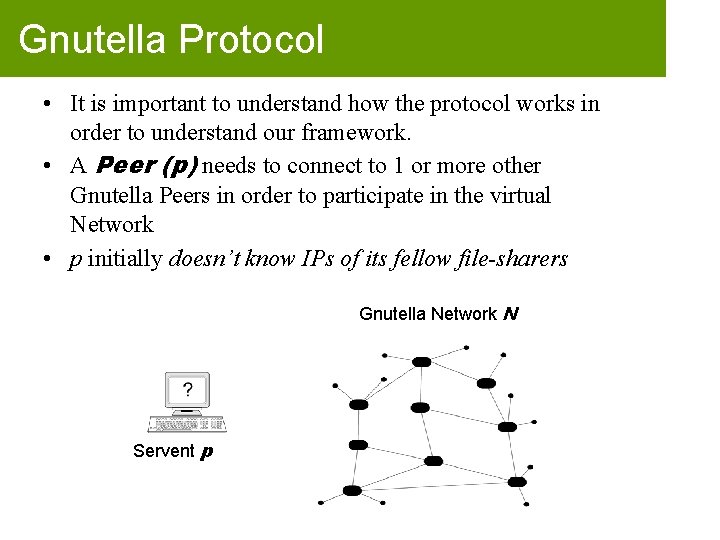
Gnutella Protocol • It is important to understand how the protocol works in order to understand our framework. • A Peer (p) needs to connect to 1 or more other Gnutella Peers in order to participate in the virtual Network • p initially doesn’t know IPs of its fellow file-sharers Gnutella Network N Servent p

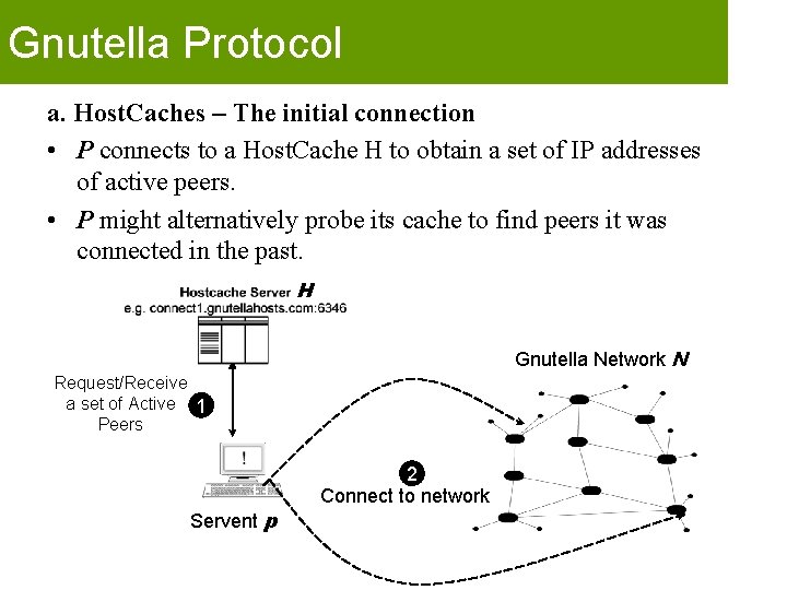
Gnutella Protocol a. Host. Caches – The initial connection • P connects to a Host. Cache H to obtain a set of IP addresses of active peers. • P might alternatively probe its cache to find peers it was connected in the past. H Gnutella Network N Request/Receive a set of Active 1 Peers Servent p 2 Connect to network

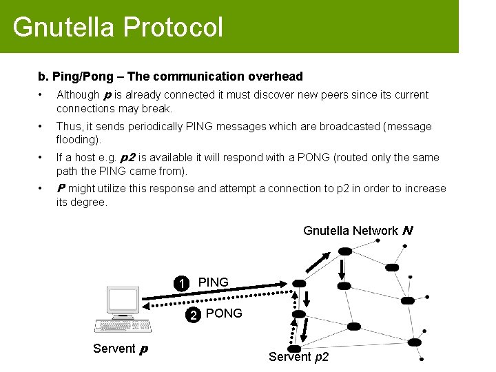
Gnutella Protocol b. Ping/Pong – The communication overhead • Although p is already connected it must discover new peers since its current connections may break. • Thus, it sends periodically PING messages which are broadcasted (message flooding). • If a host e. g. p 2 is available it will respond with a PONG (routed only the same path the PING came from). • P might utilize this response and attempt a connection to p 2 in order to increase its degree. Gnutella Network N 1 PING 2 PONG Servent p 2

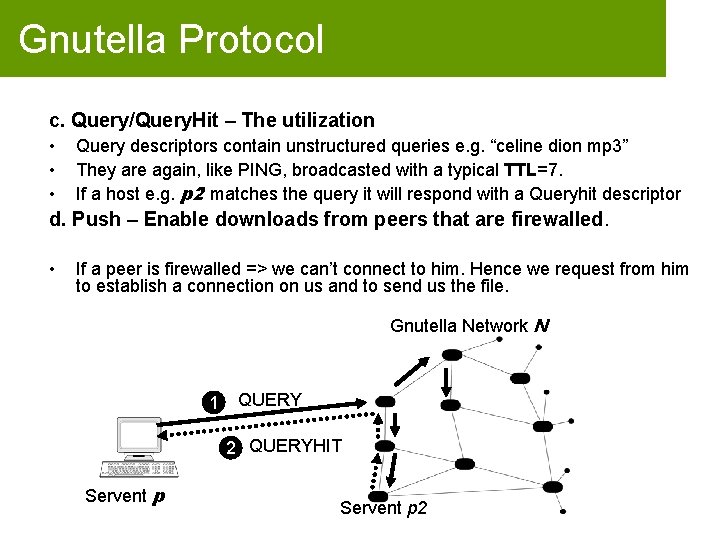
Gnutella Protocol c. Query/Query. Hit – The utilization • • • Query descriptors contain unstructured queries e. g. “celine dion mp 3” They are again, like PING, broadcasted with a typical TTL=7. If a host e. g. p 2 matches the query it will respond with a Queryhit descriptor d. Push – Enable downloads from peers that are firewalled. • If a peer is firewalled => we can’t connect to him. Hence we request from him to establish a connection on us and to send us the file. Gnutella Network N 1 QUERY 2 QUERYHIT Servent p 2

Search Performance of Gnutella • Breadth-first search always finds the optimal path • Performance is the same under random and target failure • Scales logarithmically in search path length • The search bandwidth used by query increases proportionally with the number of the nodes in the network.

Gnutella Conclusions • • • The Gnutella communication overhead is huge. Ping/Pong: 63% | Query/Query. Hits: 37%. Gnutella users can be classified in three main categories. Season-Content, Adult-Content and File Extension Searchers. Gnutella Users are mainly interested in video > audio > images > documents. Although Gnutella is a truly international phenomenon its largest segment is contributed by only a few countries. The clients started conforming to the specifications of the protocol and that they thwart excessive network resources consumption. Free riding: “Specifically, we found that nearly 70% of Gnutella users share no files, and nearly 50% of all responses are returned by the top 1% of sharing hosts”.

Advantages and Disadvantages of Centralized Indexing • Advantages: – Locates files quickly and efficiently – Searches are as comprehensive as possible – All users must registered to be on the network • Disadvantages: – Vulnerable to censorship and technical failure – Slashdot effect: popular data become less accessible because of the load of the requests on a central server – Central index might be out of data because the central server’s database is only refreshed periodically.

Advantages and Disadvantages of Decentralized Indexing • Advantages: – Inherent scalability – Avoidance of “single point of litigation” problem – Fault Tolerance • Disadvantages: – Slow information discovery – More query traffic on the network.

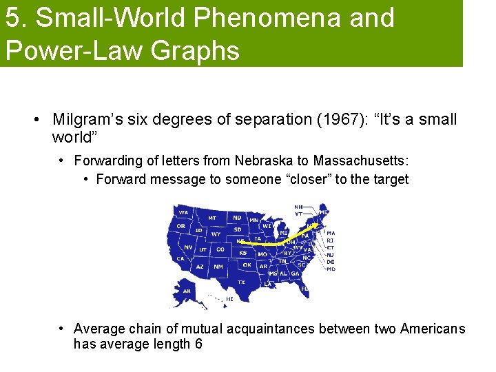
5. Small-World Phenomena and Power-Law Graphs • Milgram’s six degrees of separation (1967): “It’s a small world” • Forwarding of letters from Nebraska to Massachusetts: • Forward message to someone “closer” to the target • Average chain of mutual acquaintances between two Americans has average length 6

Small-World Phenomena and Power. Law Graphs • Power-Law Graphs – P[node has degree k] ~ for some >0 • Found in many real-life situations • Neural network of worms • AT&T Call Graph • IMDb collaboration • Gnutella • Web Graph

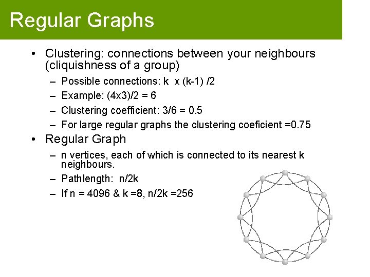
Regular Graphs • Clustering: connections between your neighbours (cliquishness of a group) – – Possible connections: k x (k-1) /2 Example: (4 x 3)/2 = 6 Clustering coefficient: 3/6 = 0. 5 For large regular graphs the clustering coeficient =0. 75 • Regular Graph – n vertices, each of which is connected to its nearest k neighbours. – Pathlength: n/2 k – If n = 4096 & k =8, n/2 k =256

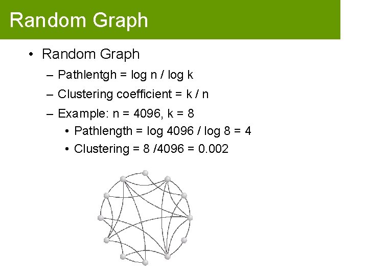
Random Graph • Random Graph – Pathlentgh = log n / log k – Clustering coefficient = k / n – Example: n = 4096, k = 8 • Pathlength = log 4096 / log 8 = 4 • Clustering = 8 /4096 = 0. 002

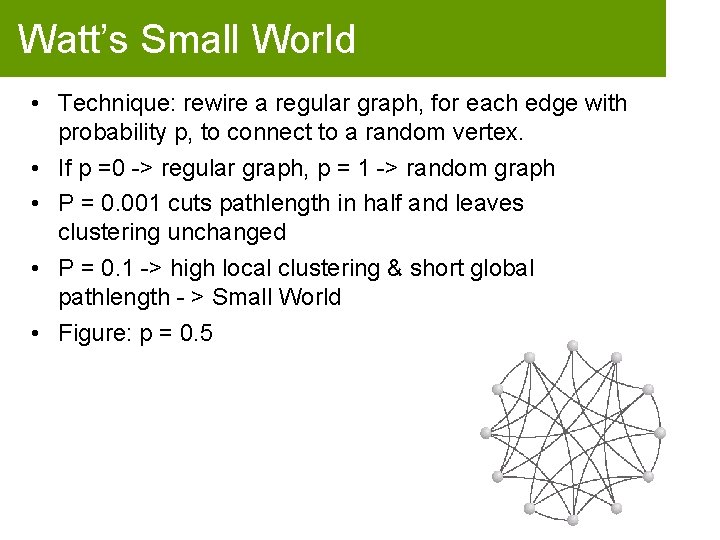
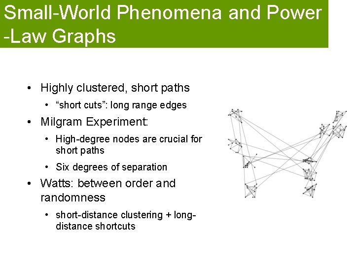
Watt’s Small World • Technique: rewire a regular graph, for each edge with probability p, to connect to a random vertex. • If p =0 -> regular graph, p = 1 -> random graph • P = 0. 001 cuts pathlength in half and leaves clustering unchanged • P = 0. 1 -> high local clustering & short global pathlength - > Small World • Figure: p = 0. 5

Small-World Phenomena and Power -Law Graphs • Highly clustered, short paths • “short cuts”: long range edges • Milgram Experiment: • High-degree nodes are crucial for short paths • Six degrees of separation • Watts: between order and randomness • short-distance clustering + longdistance shortcuts

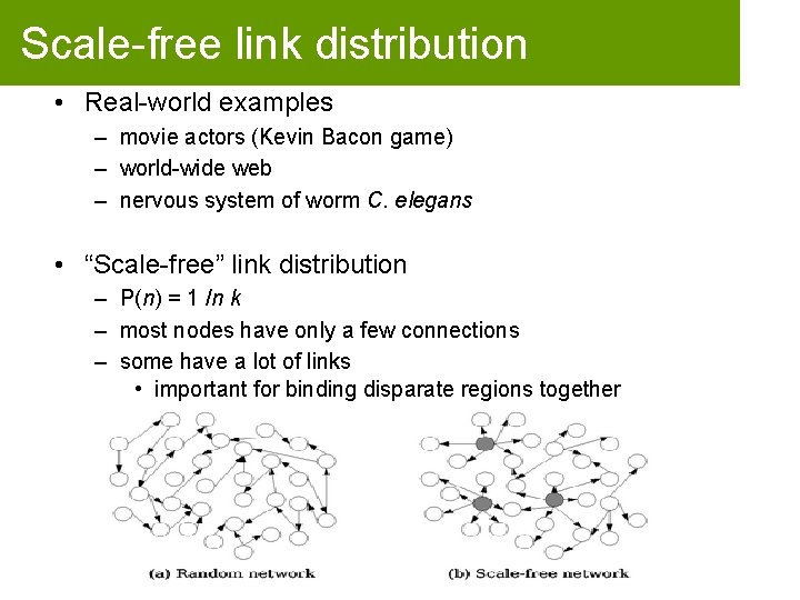
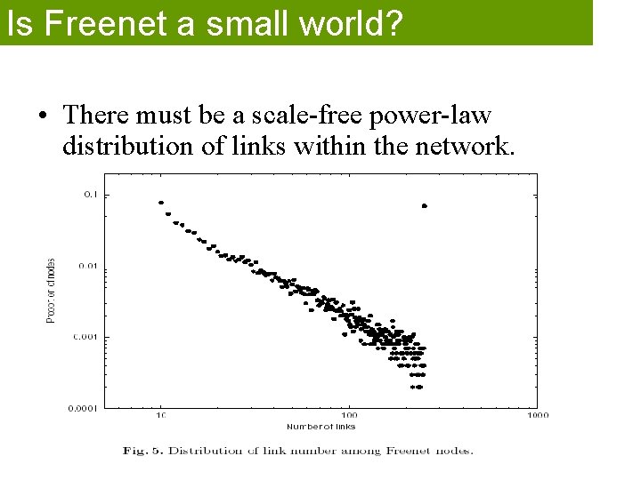
Scale-free link distribution • Real-world examples – movie actors (Kevin Bacon game) – world-wide web – nervous system of worm C. elegans • “Scale-free” link distribution – P(n) = 1 /n k – most nodes have only a few connections – some have a lot of links • important for binding disparate regions together • e. g. Tim O’Reilly

Freenet • Final Year project Ian Clarke , Edinburgh University, Scotland, June, 1999 • Sourceforge Project, most active • V. 0. 1 (released March 2000) • Latest version(Sept, 2001): 0. 4

What is Freenet and Why? • Distributed, Peer to Peer, file sharing system • Completely anonymous, for producers or consumers of information • Resistance to attempts by third parties to deny access to information

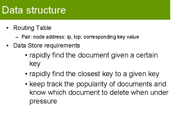
Data structure • Routing Table – Pair: node address: ip, tcp; corresponding key value • Data Store requirements • rapidly find the document given a certain key • rapidly find the closest key to a given key • keep track the popularity of documents and know which document to delete when under pressure

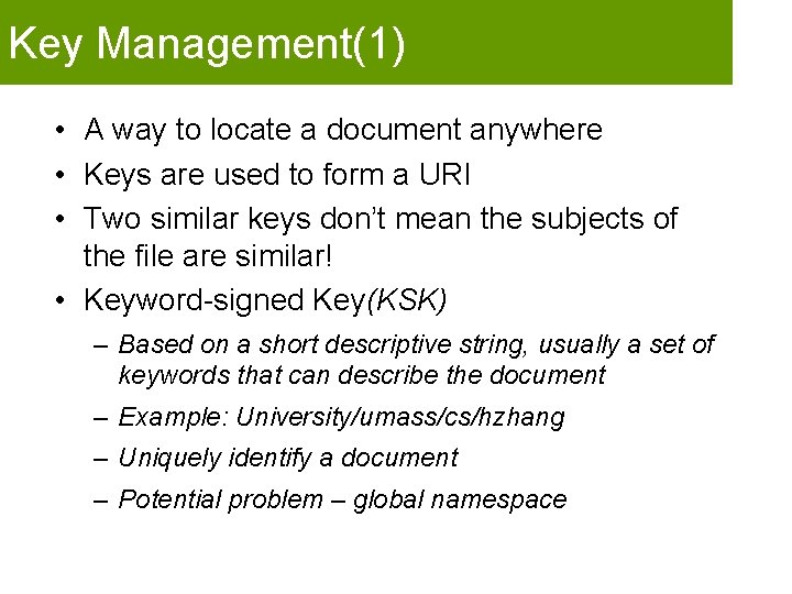
Key Management(1) • A way to locate a document anywhere • Keys are used to form a URI • Two similar keys don’t mean the subjects of the file are similar! • Keyword-signed Key(KSK) – Based on a short descriptive string, usually a set of keywords that can describe the document – Example: University/umass/cs/hzhang – Uniquely identify a document – Potential problem – global namespace

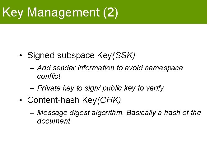
Key Management (2) • Signed-subspace Key(SSK) – Add sender information to avoid namespace conflict – Private key to sign/ public key to varify • Content-hash Key(CHK) – Message digest algorithm, Basically a hash of the document

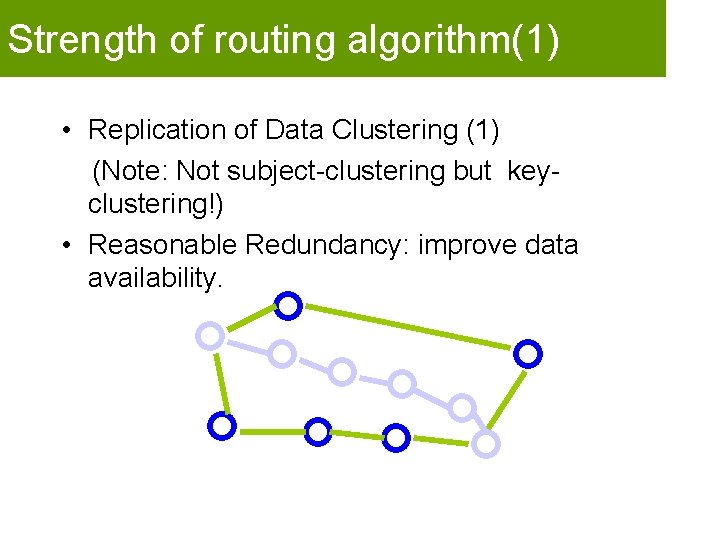
Strength of routing algorithm(1) • Replication of Data Clustering (1) (Note: Not subject-clustering but keyclustering!) • Reasonable Redundancy: improve data availability.

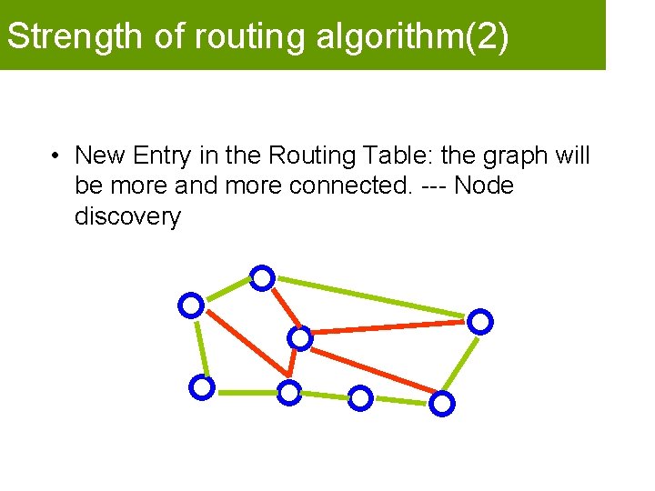
Strength of routing algorithm(2) • New Entry in the Routing Table: the graph will be more and more connected. --- Node discovery

Search Performance of Freenet • Good average case path length due to random graph property (log. N/log. K) • Poor worst-case path length due to poor local routing decisions. • Scales logarithmically • Performance suffers more in targeted attack than in random failure.

Is Freenet a small world? • There must be a scale-free power-law distribution of links within the network.

Routing in Small Worlds • Psychologist Judith Kleinfield tried to repeat Milgram’s experiment -> it didn’t work ! • Milgram’s Trick: only 98 senders were truly random, and from them only 18 letters arrived. • Problem of searching in a random small world: not a broadcast search but a directed search with insufficient information • We need distance and coordinates !!! -> Kleinberg

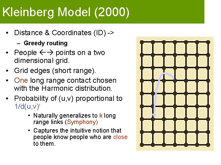
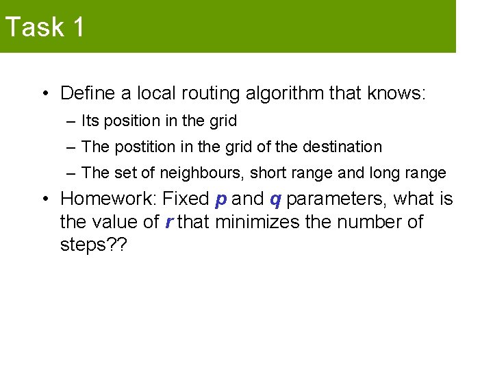
Kleinberg Model (2000) • Distance & Coordinates (ID) -> – Greedy routing • People points on a two dimensional grid. • Grid edges (short range). • One long range contact chosen with the Harmonic distribution. • Probability of (u, v) proportional to 1/d(u, v)r. • Naturally generalizes to k long range links (Symphony) • Captures the intuitive notion that people know people who are close to them.

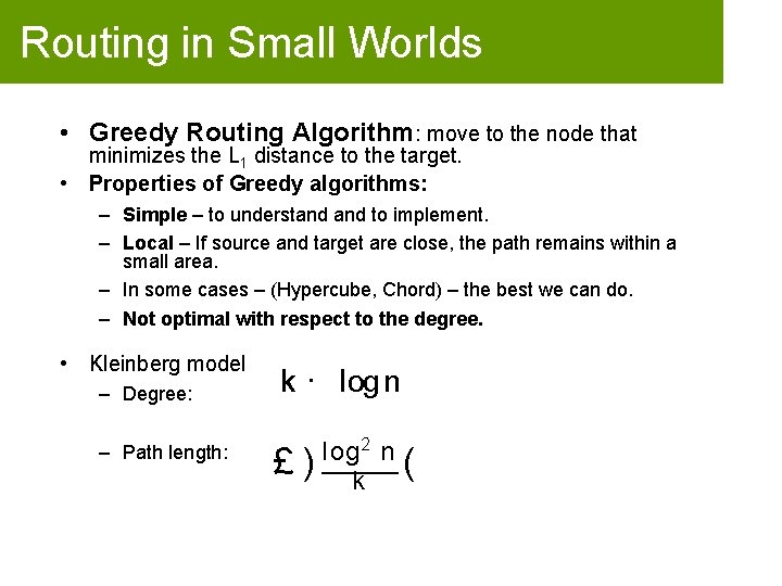
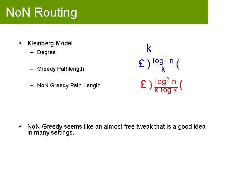
Routing in Small Worlds • Greedy Routing Algorithm: move to the node that minimizes the L 1 distance to the target. • Properties of Greedy algorithms: – Simple – to understand to implement. – Local – If source and target are close, the path remains within a small area. – In some cases – (Hypercube, Chord) – the best we can do. – Not optimal with respect to the degree. • Kleinberg model – Degree: – Path length: k · log n £ l og 2 n ) k (

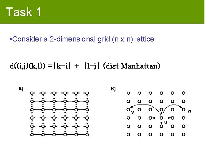
Task 1 • Consider a 2 -dimensional grid (n x n) lattice d((i, j)(k, l)) =|k-i| + |l-j| (dist Manhattan)

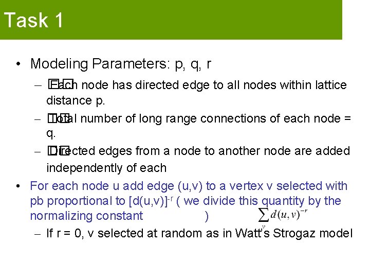
Task 1 • Modeling Parameters: p, q, r – �� Each node has directed edge to all nodes within lattice distance p. – �� Total number of long range connections of each node = q. – �� Directed edges from a node to another node are added independently of each • For each node u add edge (u, v) to a vertex v selected with pb proportional to [d(u, v)]-r ( we divide this quantity by the normalizing constant ) – If r = 0, v selected at random as in Watt’s Strogaz model

Task 1 • Define a local routing algorithm that knows: – Its position in the grid – The postition in the grid of the destination – The set of neighbours, short range and long range • Homework: Fixed p and q parameters, what is the value of r that minimizes the number of steps? ?

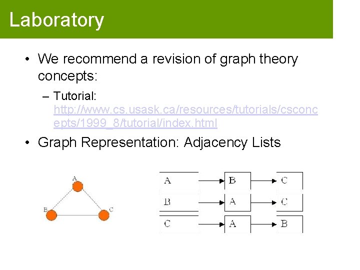
Laboratory • We recommend a revision of graph theory concepts: – Tutorial: http: //www. cs. usask. ca/resources/tutorials/csconc epts/1999_8/tutorial/index. html • Graph Representation: Adjacency Lists

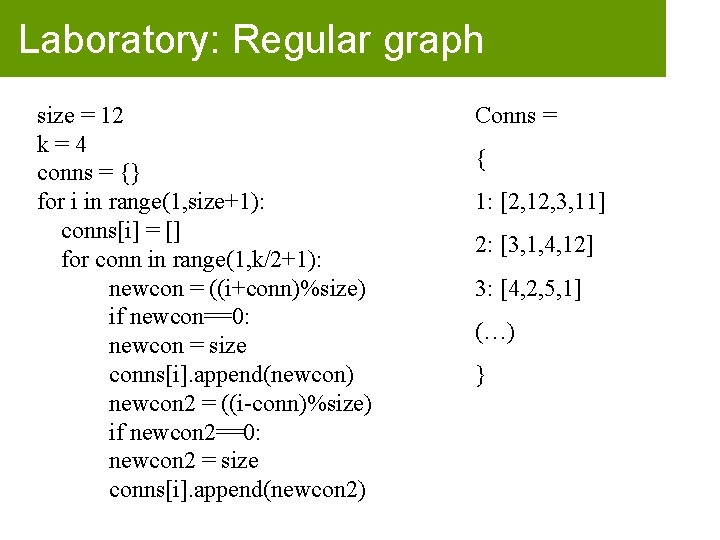
Laboratory: Regular graph size = 12 k=4 conns = {} for i in range(1, size+1): conns[i] = [] for conn in range(1, k/2+1): newcon = ((i+conn)%size) if newcon==0: newcon = size conns[i]. append(newcon) newcon 2 = ((i-conn)%size) if newcon 2==0: newcon 2 = size conns[i]. append(newcon 2) Conns = { 1: [2, 12, 3, 11] 2: [3, 1, 4, 12] 3: [4, 2, 5, 1] (…) }

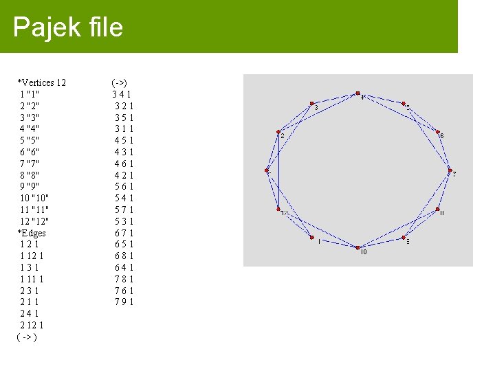
Pajek file *Vertices 12 1 "1" 2 "2" 3 "3" 4 "4" 5 "5" 6 "6" 7 "7" 8 "8" 9 "9" 10 "10" 11 "11" 12 "12" *Edges 121 1 12 1 131 1 11 1 231 211 241 2 12 1 ( -> ) (->) 341 321 351 311 451 431 461 421 561 541 571 531 671 651 681 641 781 761 791

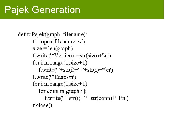
Pajek Generation def to. Pajek(graph, filename): f = open(filename, 'w') size = len(graph) f. write('*Vertices '+str(size)+'n') for i in range(1, size+1): f. write(' '+str(i)+' "'+str(i)+'"n') f. write('*Edgesn') for i in range(1, size+1): for conn in graph[i]: f. write(' '+str(i)+' '+str(conn)+' 1n') f. close()

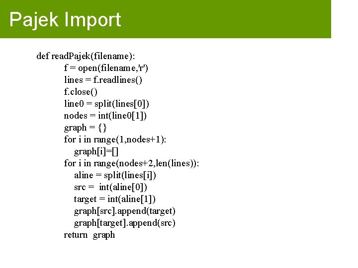
Pajek Import def read. Pajek(filename): f = open(filename, 'r') lines = f. readlines() f. close() line 0 = split(lines[0]) nodes = int(line 0[1]) graph = {} for i in range(1, nodes+1): graph[i]=[] for i in range(nodes+2, len(lines)): aline = split(lines[i]) src = int(aline[0]) target = int(aline[1]) graph[src]. append(target) graph[target]. append(src) return graph

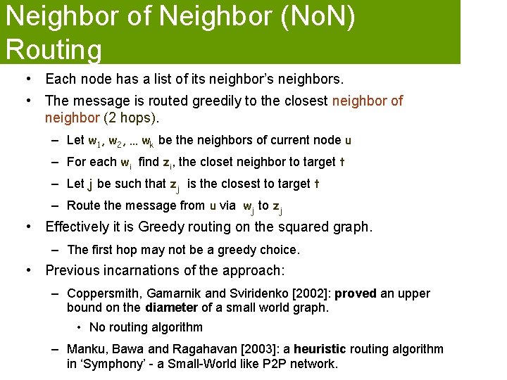
Neighbor of Neighbor (No. N) Routing • Each node has a list of its neighbor’s neighbors. • The message is routed greedily to the closest neighbor of neighbor (2 hops). – Let w 1, w 2, … wk be the neighbors of current node u – For each wi find zi, the closet neighbor to target t – Let j be such that zj is the closest to target t – Route the message from u via wj to zj • Effectively it is Greedy routing on the squared graph. – The first hop may not be a greedy choice. • Previous incarnations of the approach: – Coppersmith, Gamarnik and Sviridenko [2002]: proved an upper bound on the diameter of a small world graph. • No routing algorithm – Manku, Bawa and Ragahavan [2003]: a heuristic routing algorithm in ‘Symphony’ - a Small-World like P 2 P network.

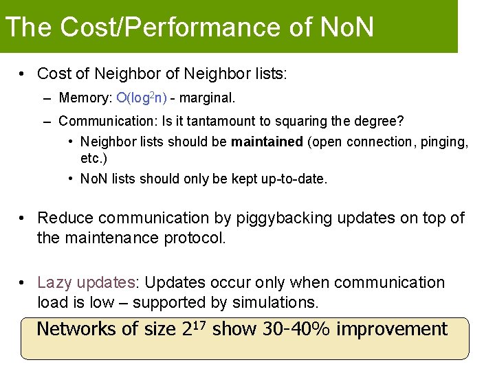
The Cost/Performance of No. N • Cost of Neighbor lists: – Memory: O(log 2 n) - marginal. – Communication: Is it tantamount to squaring the degree? • Neighbor lists should be maintained (open connection, pinging, etc. ) • No. N lists should only be kept up-to-date. • Reduce communication by piggybacking updates on top of the maintenance protocol. • Lazy updates: Updates occur only when communication load is low – supported by simulations. Networks of size 217 show 30 -40% improvement

No. N Routing • Kleinberg Model – Degree – Greedy Pathlength – No. N Greedy Path Length k l og 2 n £) k ( £ l og 2 n ) k l og k ( • No. N Greedy seems like an almost free tweak that is a good idea in many settings.

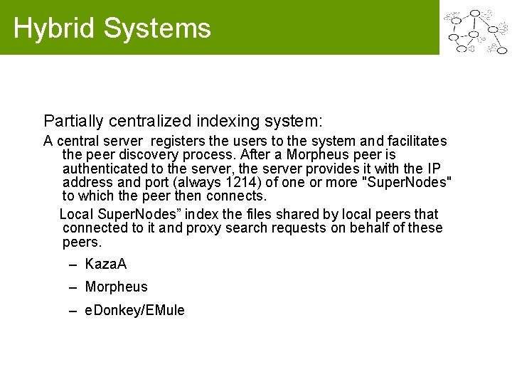
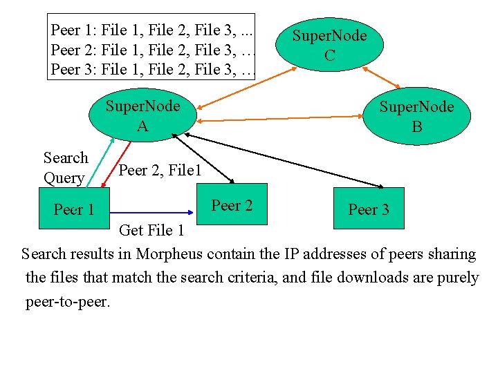
Hybrid Systems Partially centralized indexing system: A central server registers the users to the system and facilitates the peer discovery process. After a Morpheus peer is authenticated to the server, the server provides it with the IP address and port (always 1214) of one or more "Super. Nodes" to which the peer then connects. Local Super. Nodes” index the files shared by local peers that connected to it and proxy search requests on behalf of these peers. – Kaza. A – Morpheus – e. Donkey/EMule

Peer 1: File 1, File 2, File 3, . . . Peer 2: File 1, File 2, File 3, … Peer 3: File 1, File 2, File 3, … Super. Node A Search Query Peer 1 Super. Node C Super. Node B Peer 2, File 1 Peer 2 Peer 3 Get File 1 Search results in Morpheus contain the IP addresses of peers sharing the files that match the search criteria, and file downloads are purely peer-to-peer.

Morpheus’s Super. Node • Morpheus peers are automatically elected to become Super. Nodes if they have sufficient bandwidth and processing power (a configuration parameter allows users to opt out of running their peer in this mode). • Once a Morpheus peer receives its list of Super. Nodes from the central server, little communication with the server is required.

Advantages of Partial Centralized Indexing • Reducing discovery time in comparison with purely decentralized indexing system such as Gnutella and Freenet • Reducing the workload on central servers in comparison with fully centralized indexing system such as Napster.

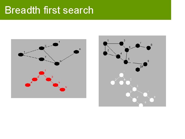
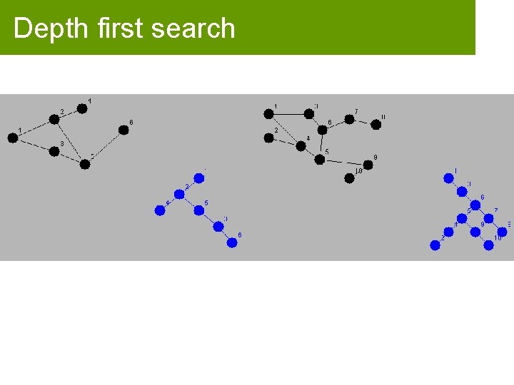
6. Data Location • Gnutella: : BFS (Breadth First Search) – A node sends query to all its neighbors and each neighbor searches itself and forwards the message to all its own neighbors – If (once) query is satisfied, response sent back to the original requester – Can cause a lot of traffic – Query Flooding • Freenet: DFS (Depth First Search) – Each file has a unique ID and location – Information stored on peer host under searchable keys – Depth-first search—each node forwards the query to a single neighbor – If query not satisfied, forwards query to another neighbor

Breadth first search

Depth first search

P 2 P Search • Gnutella: BFS technique is used with depth limit of D, where D= TTL of the message. At all levels <D query is processed by each node and results are sent to source and at level D query is dropped. • Freenet: uses DFS with depth limit D. Each node forwards the query to a single neighbor and waits for a definite response from the neighbor before forwarding the query to another neighbor(if the query was not satisfied), or forwarding the results back to the query source(if query was satisfied).

P 2 P Search • Quality of results measured only by number of results then BFS is ideal • If Satisfaction is metrics of choice BFS wastes much bandwidth and processing power • With DFS each node processes the query sequentially, searches can be terminated as soon as the query is satisfied, thereby minimizing cost. But poor response time due to the above

P 2 P Search Algorithms • Directed BFS – Node sends query to a subset of its neighbors and waits either for a minimum number of results or for a maximum amount of time – Node keeps info on its neighbors from past queries for better searching in the future – Node also keeps info on the speed and connection time of its neighbor – Can know which neighbor has highest/lowest number of results – Neighbors that forwards many/few messages • Local Indices – Each node maintains index of data of all nodes w/in a certain amount of distance from itself…. a “radius” – When receives a query, a node can process it on behalf of itself or for every node within its radius…. fewer nodes to be searched

Replication and Epidemics • Key idea was that p 2 p systems could “gossip” about replicated data – Now and then, each node picks some “peer” (at random, more or less) – Sends it a snapshot of its own data • Called “push gossip” – Or asks for a snapshot of the peer’s data • “Pull” gossip – Or both: a push-pull interaction

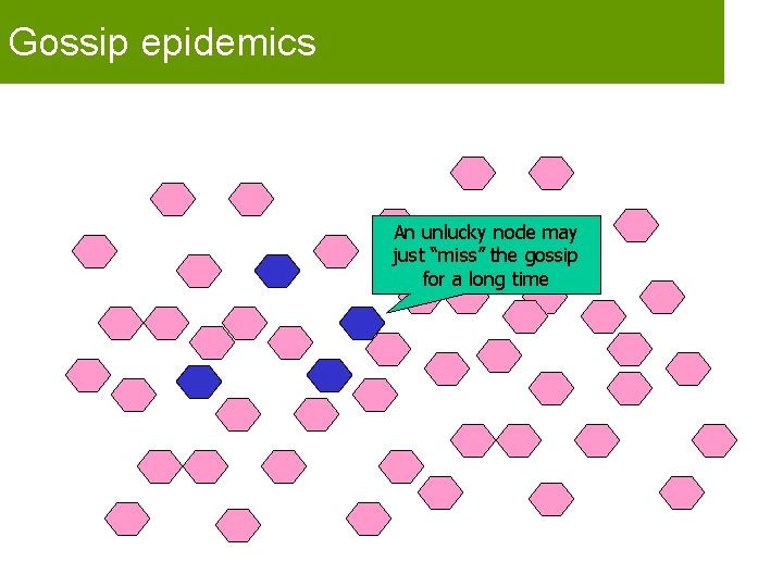
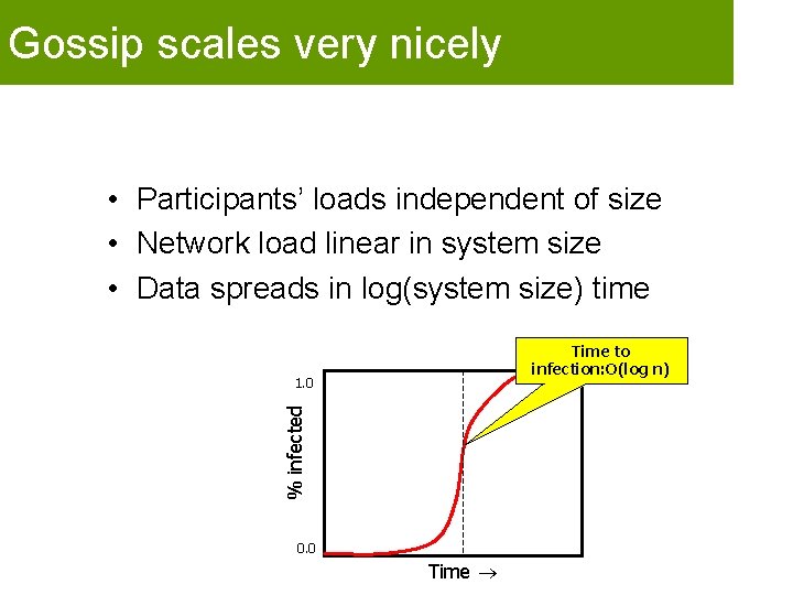
Gossip “epidemics” – [t=0] Suppose that I know something – [t=1] I pick you… Now two of us know it. – [t=2] We each pick … now 4 know it… • Information spread: exponential rate. – Due to re-infection (gossip to an infected node) spreads as 1. 8 k after k rounds – But in O(log(N)) time, N nodes are infected

Gossip epidemics An unlucky node may just “miss” the gossip for a long time

Gossip scales very nicely • Participants’ loads independent of size • Network load linear in system size • Data spreads in log(system size) time Time to infection: O(log n) % infected 1. 0 0. 0 Time

Facts about gossip epidemics • Extremely robust – Data travels on exponentially many paths! – Hard to even slow it down… • Suppose 50% of our packets are simply lost… • … we’ll need 1 additional round: a trivial delay! – Push-pull works best. For push-only/pull-only a few nodes can remain uninfected for a long time

Uses of gossip epidemics • To robustly multicast data – Slow, but very sure of getting through • To repair inconsistency in replicas • To support “all to all” monitoring and distributed management • For distributed data mining and discovery

Laboratory def infect (node, infected, graph): newvictims = [] for victim in graph[node]: if not(infected. __contains__(victim)): newvictims. append(victim) return newvictims

Laboratory def epidemics (src, graph, time): if time==0: infected = [src] infected = infected + infect (src, infected, graph) return infected else: infected = [src] infected = infected + infect (src, infected, graph) result = [] for i in range(time): for node in infected: result = concat (result, infect (node, infected, graph)) infected = infected + result return infected

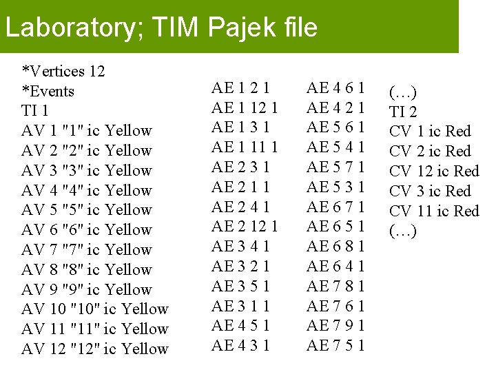
Laboratory; TIM Pajek file *Vertices 12 *Events TI 1 AV 1 "1" ic Yellow AV 2 "2" ic Yellow AV 3 "3" ic Yellow AV 4 "4" ic Yellow AV 5 "5" ic Yellow AV 6 "6" ic Yellow AV 7 "7" ic Yellow AV 8 "8" ic Yellow AV 9 "9" ic Yellow AV 10 "10" ic Yellow AV 11 "11" ic Yellow AV 12 "12" ic Yellow AE 1 2 1 AE 1 12 1 AE 1 3 1 AE 1 11 1 AE 2 3 1 AE 2 1 1 AE 2 4 1 AE 2 12 1 AE 3 4 1 AE 3 2 1 AE 3 5 1 AE 3 1 1 AE 4 5 1 AE 4 3 1 AE 4 6 1 AE 4 2 1 AE 5 6 1 AE 5 4 1 AE 5 7 1 AE 5 3 1 AE 6 7 1 AE 6 5 1 AE 6 8 1 AE 6 4 1 AE 7 8 1 AE 7 6 1 AE 7 9 1 AE 7 5 1 (…) TI 2 CV 1 ic Red CV 2 ic Red CV 12 ic Red CV 3 ic Red CV 11 ic Red (…)

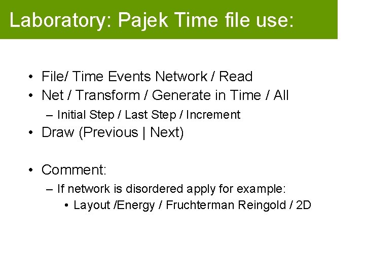
Laboratory: Pajek Time file use: • File/ Time Events Network / Read • Net / Transform / Generate in Time / All – Initial Step / Last Step / Increment • Draw (Previous | Next) • Comment: – If network is disordered apply for example: • Layout /Energy / Fruchterman Reingold / 2 D

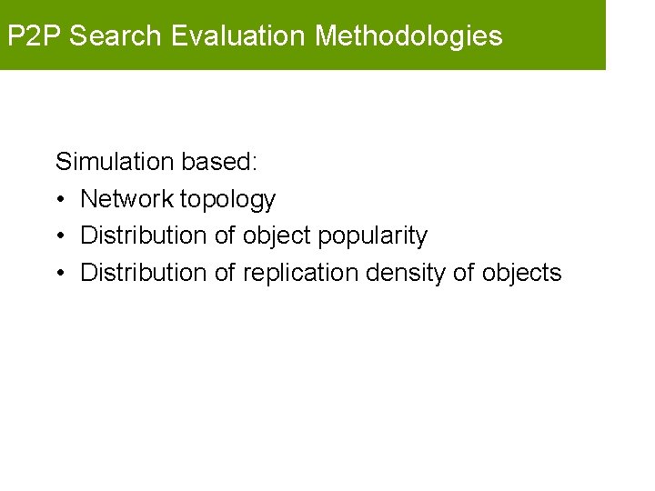
P 2 P Search Evaluation Methodologies Simulation based: • Network topology • Distribution of object popularity • Distribution of replication density of objects

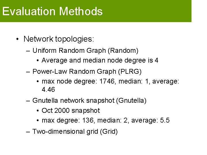
Evaluation Methods • Network topologies: – Uniform Random Graph (Random) • Average and median node degree is 4 – Power-Law Random Graph (PLRG) • max node degree: 1746, median: 1, average: 4. 46 – Gnutella network snapshot (Gnutella) • Oct 2000 snapshot • max degree: 136, median: 2, average: 5. 5 – Two-dimensional grid (Grid)

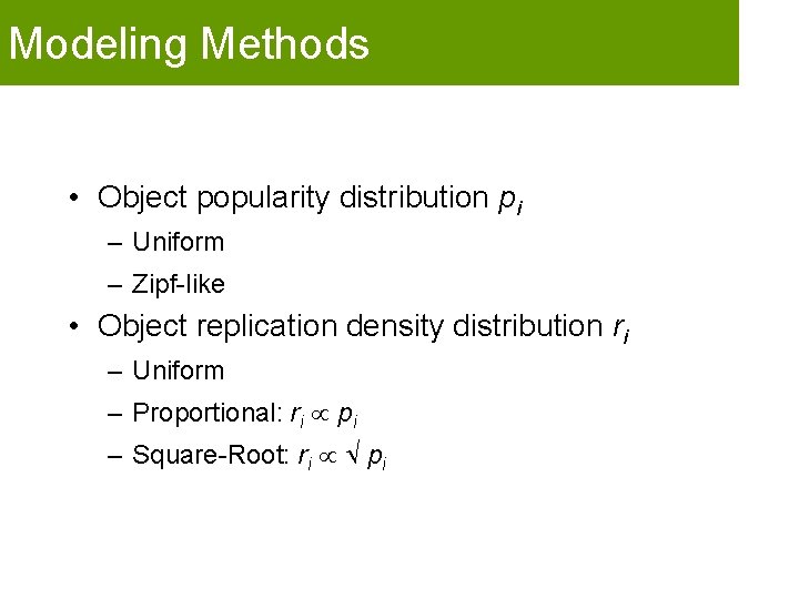
Modeling Methods • Object popularity distribution pi – Uniform – Zipf-like • Object replication density distribution ri – Uniform – Proportional: ri pi – Square-Root: ri pi

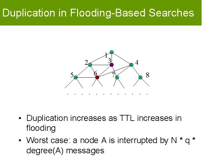
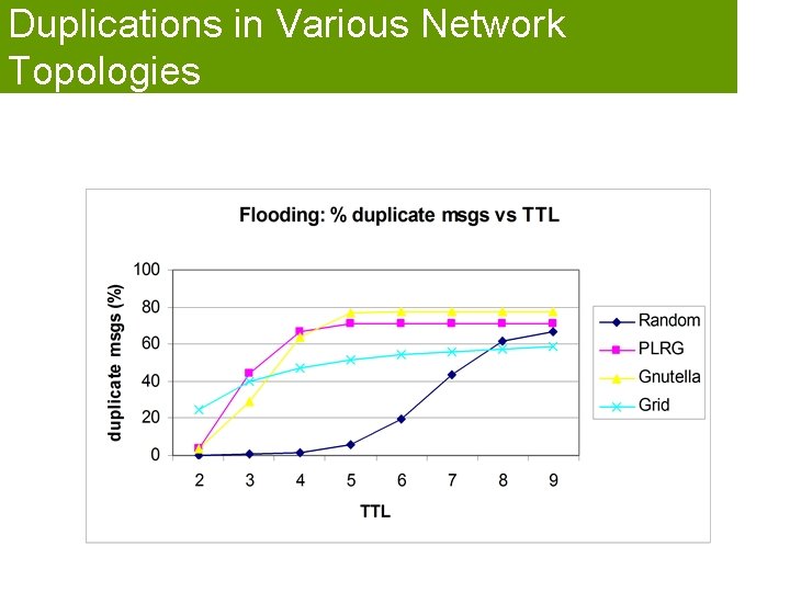
Duplication in Flooding-Based Searches 1 3 2 5 6 4 7 8 . . . • Duplication increases as TTL increases in flooding • Worst case: a node A is interrupted by N * q * degree(A) messages

Duplications in Various Network Topologies

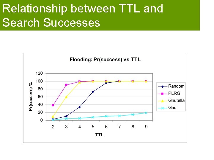
Relationship between TTL and Search Successes

Problems with Simple TTL-Based Flooding • Hard to choose TTL: – For objects that are widely present in the network, small TTLs suffice – For objects that are rare in the network, large TTLs are necessary • Number of query messages grow exponentially as TTL grows

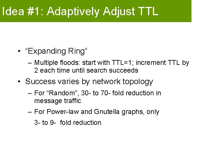
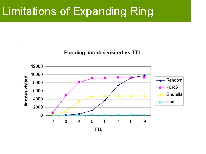
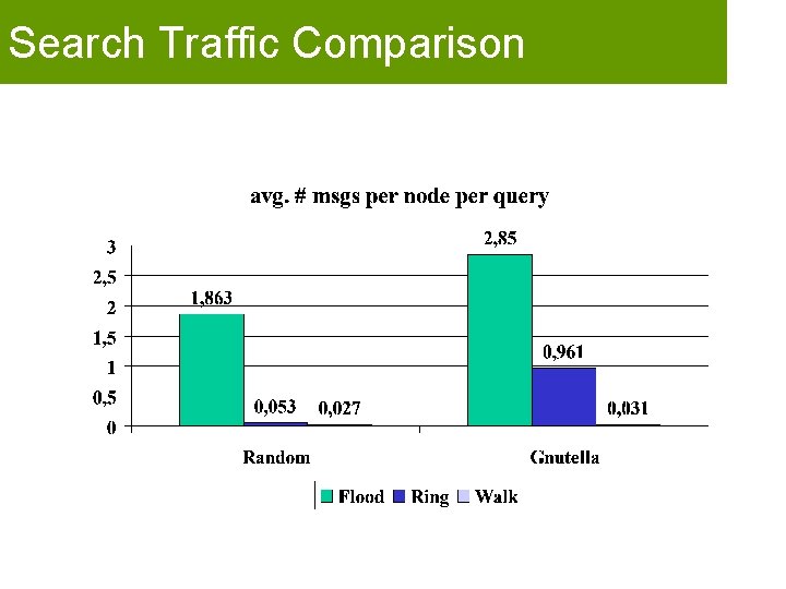
Idea #1: Adaptively Adjust TTL • “Expanding Ring” – Multiple floods: start with TTL=1; increment TTL by 2 each time until search succeeds • Success varies by network topology – For “Random”, 30 - to 70 - fold reduction in message traffic – For Power-law and Gnutella graphs, only 3 - to 9 - fold reduction

Limitations of Expanding Ring

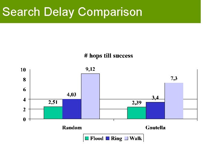
Idea #2: Random Walk • Simple random walk – takes too long to find anything! • Multiple-walker random walk – N agents after each walking T steps visits as many nodes as 1 agent walking N*T steps – When to terminate the search: check back with the query originator once every C steps

Search Traffic Comparison

Search Delay Comparison

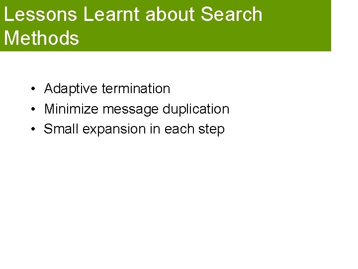
Lessons Learnt about Search Methods • Adaptive termination • Minimize message duplication • Small expansion in each step

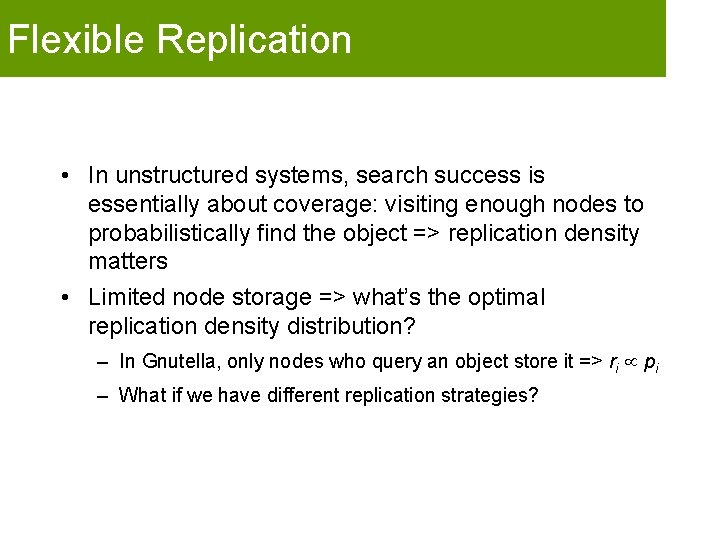
Flexible Replication • In unstructured systems, search success is essentially about coverage: visiting enough nodes to probabilistically find the object => replication density matters • Limited node storage => what’s the optimal replication density distribution? – In Gnutella, only nodes who query an object store it => ri pi – What if we have different replication strategies?

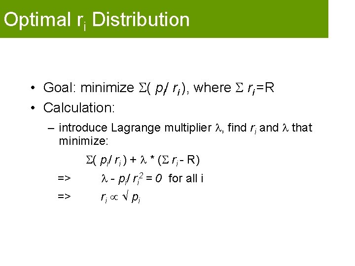
Optimal ri Distribution • Goal: minimize ( pi/ ri ), where ri =R • Calculation: – introduce Lagrange multiplier , find ri and that minimize: ( pi/ ri ) + * ( ri - R) => - pi/ ri 2 = 0 for all i => ri p i

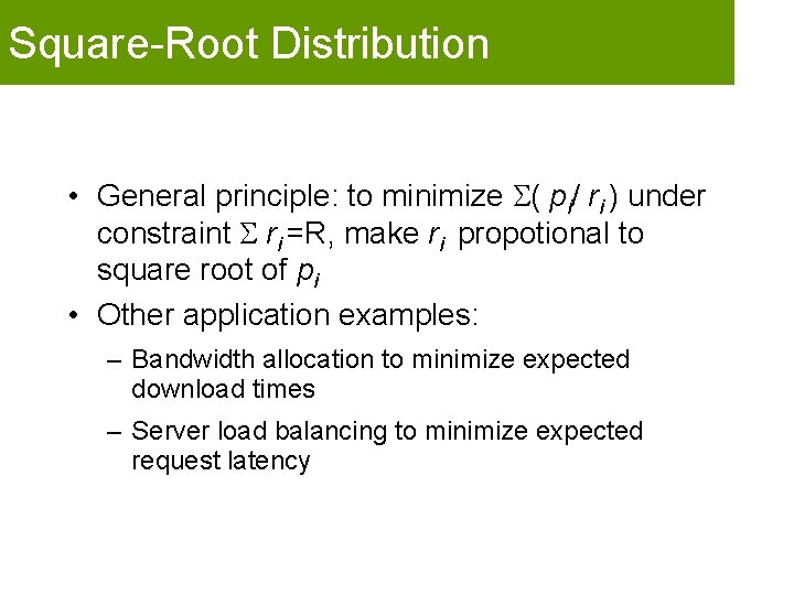
Square-Root Distribution • General principle: to minimize ( pi/ ri ) under constraint ri =R, make ri propotional to square root of pi • Other application examples: – Bandwidth allocation to minimize expected download times – Server load balancing to minimize expected request latency

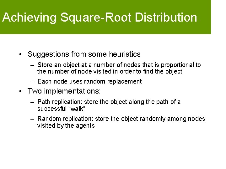
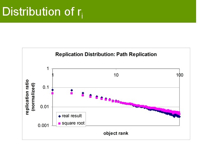
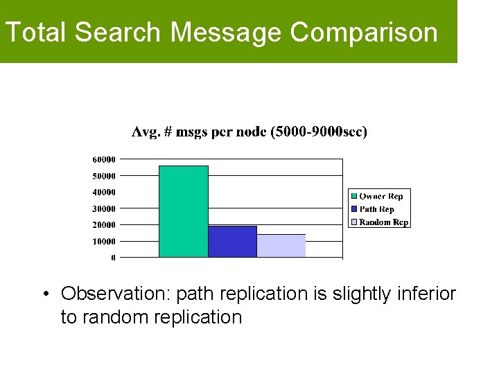
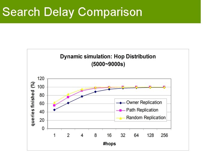
Achieving Square-Root Distribution • Suggestions from some heuristics – Store an object at a number of nodes that is proportional to the number of node visited in order to find the object – Each node uses random replacement • Two implementations: – Path replication: store the object along the path of a successful “walk” – Random replication: store the object randomly among nodes visited by the agents

Distribution of ri

Total Search Message Comparison • Observation: path replication is slightly inferior to random replication

Search Delay Comparison

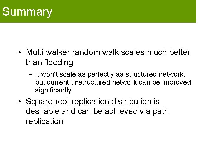
Summary • Multi-walker random walk scales much better than flooding – It won’t scale as perfectly as structured network, but current unstructured network can be improved significantly • Square-root replication distribution is desirable and can be achieved via path replication

Conclusions • Towards Structured P 2 P Networks, See you in the next lesson !