OVERVIEW Omer Berkman 1 Contents n n n

OVERVIEW Omer Berkman 1

Contents n n n Biological background Using Gene-arrays to decipher generegulatory interactions Applications… 2

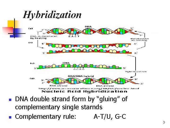
Hybridization n n DNA double strand form by “gluing” of complementary single starnds Complementary rule: A-T/U, G-C 3

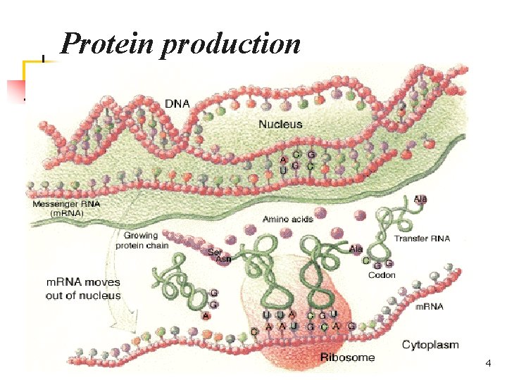
Protein production 4

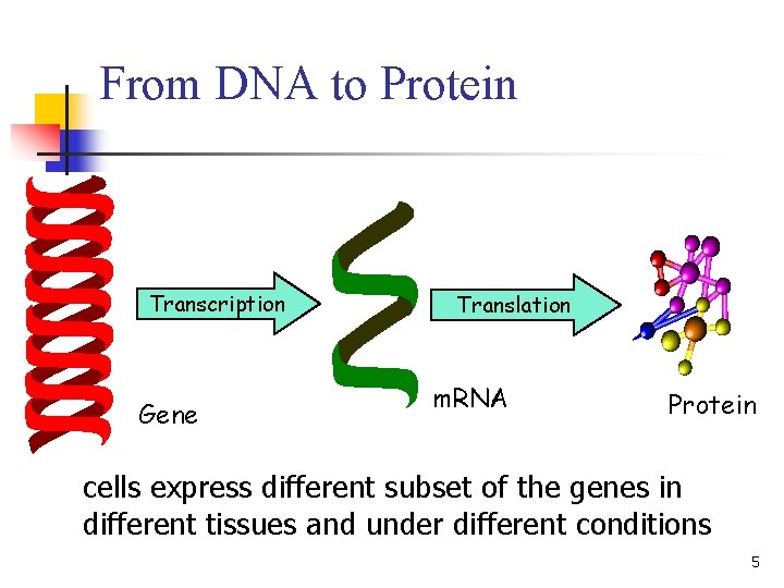
From DNA to Protein Transcription Gene Translation m. RNA Protein cells express different subset of the genes in different tissues and under different conditions 5

Functional genomics n n The complete sequences of many microbial genomes are already known - the inventory of the building blocks of life was collected. next stage is ‘‘re-assembling the pieces’’ : n Defining the role of each gene in these genomes. n Understanding how the genome functions as a whole in the complex natural history of a living organism. Knowing when and where a gene is expressed often provides a strong clue as to its biological role 6

Transcriptional process n n This process is highly regulated. One of the most important ways in which the cell regulates gene expression is by using a feedback loop. some of the proteins are transcription factors. These proteins regulate the expression of other genes (and possibly, their own expression) by either initiating or repressing 7 transcription.

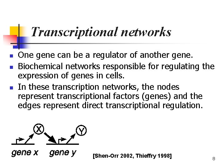
Transcriptional networks n n n One gene can be a regulator of another gene. Biochemical networks responsible for regulating the expression of genes in cells. In these transcription networks, the nodes represent transcriptional factors (genes) and the edges represent direct transcriptional regulation. [Shen-Orr 2002, Thieffry 1998] 8

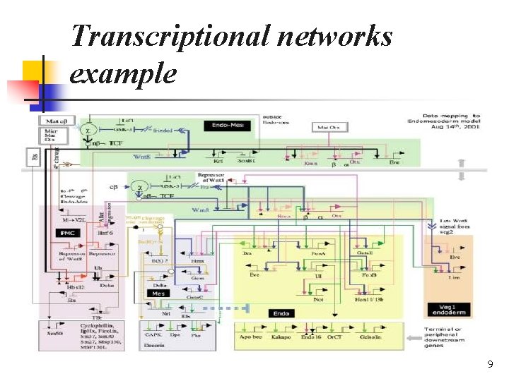
Transcriptional networks example 9

Gene-arrays for m. RNA analysis n n n Differences in cell type or state are correlated with changes in the m. RNA levels of its genes. The only specific reagent required to measure the abundance of the m. RNA for a specific gene is a c. DNA sequence. DNA microarrays provide a practical and economical tool for studying gene expression on a very large scale. 10

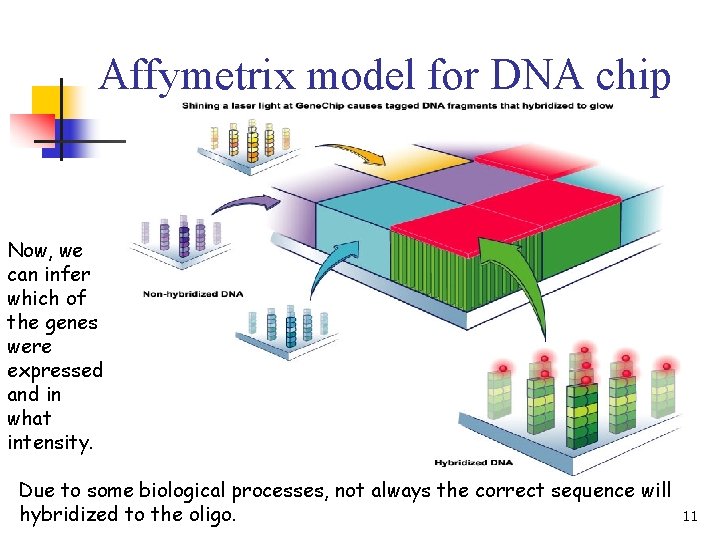
Affymetrix model for DNA chip Now, we can infer which of the genes were expressed and in what intensity. Due to some biological processes, not always the correct sequence will hybridized to the oligo. 11

Gene Arrays / DNA chips n n n From “one gene in one experiment” to “massively parallel biological data acquisition”. Simultaneously analyzing the expression levels of large numbers of genes provides the opportunity to study the activity of whole genomes. Large-scale gene expression analysis reveals the behavior of co-regulated gene networks. 12

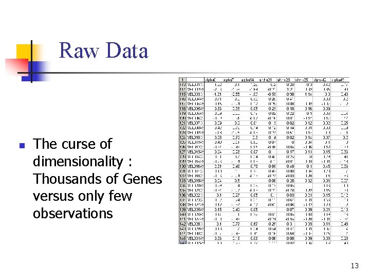
Raw Data n The curse of dimensionality : Thousands of Genes versus only few observations 13

Static versus dynamic We distinguish between static experiments and time series experiments: n Static – n n n A snapshot in different samples is measured. Data are assumed to be independent identically distributed. Dynamic – n n A temporal process is measured. Data have strong autocorrelation between successive points. 14

Temporal observations n n n It’s possible to produce time-dependent measurements, termed expression matrices. These expression matrices are the result of the underlying regulatory network. Reverse engineering seeks to extract information from time-series measurements in order to identify regulatory interactions in these genetic networks. 15

Complications n n n n The curse of dimensionality Extremely noisy observations Expensive experiments Stochastic nature Population averaged Feasible time scale Partially information We are facing a hard problem… 16

1. The curse of dimensionality (Bellman, 1961) n n n The number of genes typically far exceeds the number of time points for which data are available, making the problem an ill-posed one. “Traditional statistics” won’t help here - the amount of samples, versus the number of genes, does not provide enough information to construct a full detailed model with high statistical significance. New statistical methods/approaches were developed (Bootstrap, Interpolations, Clustering, FDR…) 17

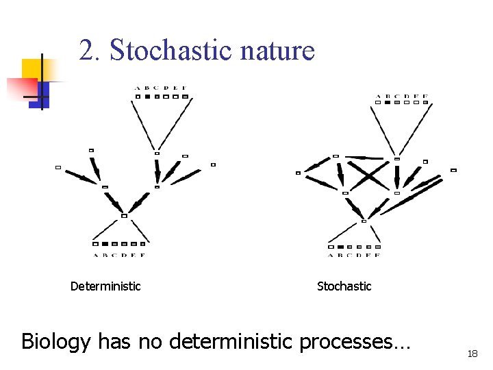
2. Stochastic nature Deterministic Stochastic Biology has no deterministic processes… 18

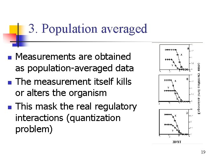
3. Population averaged n n n Measurements are obtained as population-averaged data The measurement itself kills or alters the organism This mask the real regulatory interactions (quantization problem) 19

4. Feasible time scale Empirical limit on the number of time points : n n The average speed of the biologic process determines the number of informative points. The error of the method applied have to be smaller than the expression level difference. MISSING REGULATORY INTERACTIONS COST and ERROR 20

5. Partial information n n Biological systems are robust, adaptable, and redundant. Genes are not the only actor in the game – transcriptional factors can be of many kinds. The regulatory interactions between genes are not deterministic at the m. RNA level - a gene has few independently regulated derivatives. m. RNA expression data alone only gives a partial picture that does not reflect key events such as 21 translation and protein (in)activation.

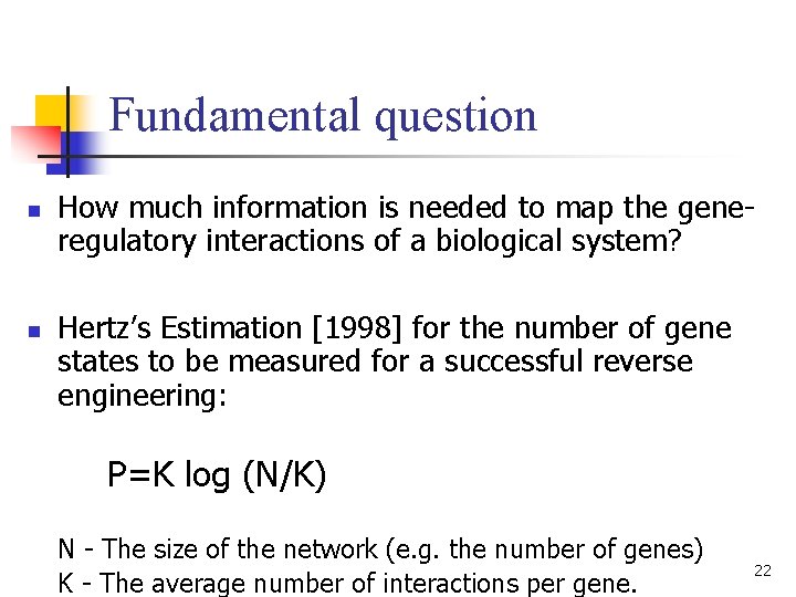
Fundamental question n n How much information is needed to map the generegulatory interactions of a biological system? Hertz’s Estimation [1998] for the number of gene states to be measured for a successful reverse engineering: P=K log (N/K) N - The size of the network (e. g. the number of genes) K - The average number of interactions per gene. 22

Application 1 [De. Risi 1997] Exploring the metabolic and genetic control of gene expression n n Investigation of gene expression accompanying the metabolic shift from fermentation to respiration in yeast. Identify genes whose expression was affected by deletion of TUP 1 or overexpression of YAP 1. 23

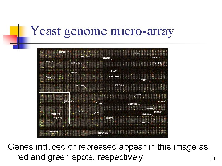
Yeast genome micro-array Genes induced or repressed appear in this image as red and green spots, respectively. 24

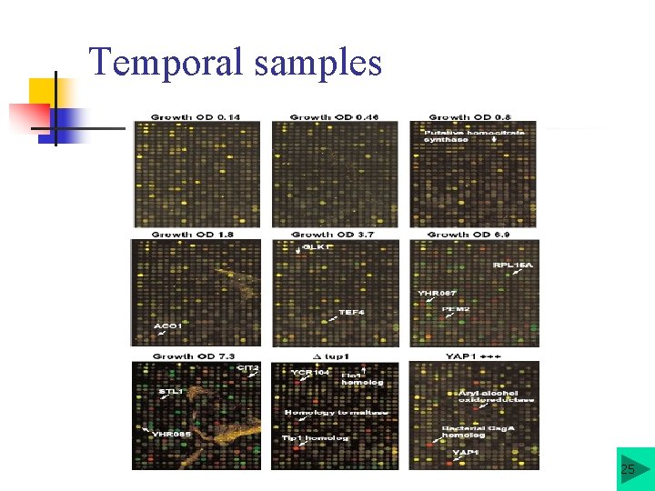
Temporal samples 25

Analysis n n Stable gene expression during exponential growth. A marked change was seen as glucose was progressively depleted from the growth media. - m. RNA levels for 710 genes were induced. - m. RNA levels for 1030 genes declined. The expression patterns observed for previously characterized genes showed concordance with previously published results. About half of these differentially expressed genes have no apparent homology to any gene whose function is 26 known. This provides the first small clue to their

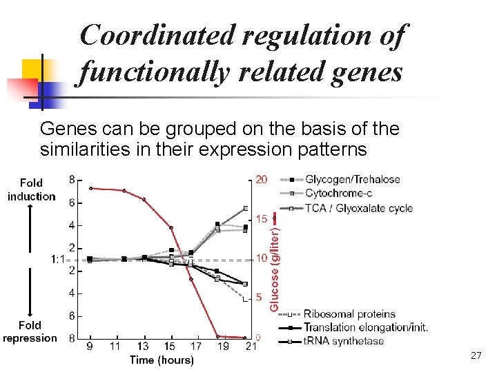
Coordinated regulation of functionally related genes Genes can be grouped on the basis of the similarities in their expression patterns 27

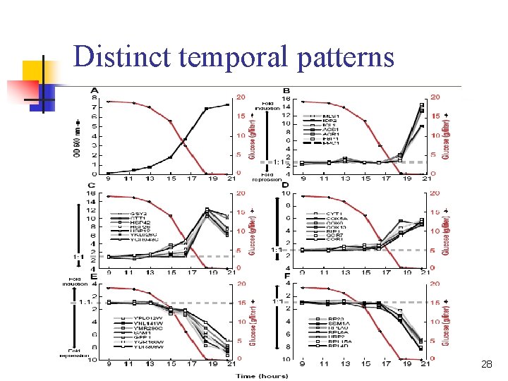
Distinct temporal patterns 28

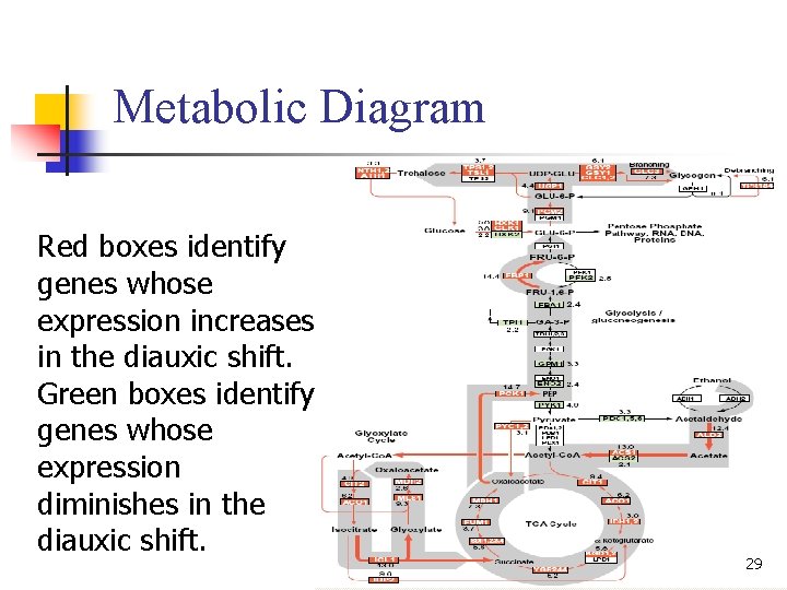
Metabolic Diagram Red boxes identify genes whose expression increases in the diauxic shift. Green boxes identify genes whose expression diminishes in the diauxic shift. 29

Defining the contributions of individual regulatory genes n n Using a DNA micro-array to identify genes whose expression is affected by mutations in each putative regulatory gene. Performing: - Deletion the transcriptional repressor TUP 1. - Overexpression of the transcriptional activator YAP 1. 30

Deleting the TUP 1 gene n n Wild-type yeast cells and cells bearing a deletion of the TUP 1 gene were grown. m. RNA was isolated from the two populations and used to prepare c-DNA labeled with green and red. The labeled probes were mixed and simultaneously hybridized to the micro-array. Red spots on the array represent genes that were induced in the TUP 1 strain, and thus presumably repressed by TUP 1. 31

Overexpressing the YAP 1 gene n n Complementary DNA from the control and YAP 1 over-expressing strains, labeled with Cy 3 and Cy 5, respectively, was prepared from m. RNA isolated from the two strains and hybridized to the micro-array. Red spots on the array represent genes that were induced in the strain overexpressing YAP 1. 32

Characterization of regulatory pathways and networks n n n Use of a micro-array to characterize the transcriptional consequences of mutations provides a simple and powerful approach. This strategy also has an important practical application in drug screening. However, one should keep in mind that transcriptional regulations might be complicated. 33

Application 1 summary n n n DNA micro-arrays provide a simple and economical way to explore gene expression patterns on a genomic scale. “The greatest challenge now is to develop efficient methods for organizing, interpreting, and extracting insights from the large volumes of data these experiments provide. ” Technical advances have made array experiments fairly easy to do, but tools for analysis of data produced have lagged behind. 34

Application 2 [Friedman 2000] Using Bayesian Networks to Analyze Expression Data n n Probabilistic approach. Bayesian network as a model for genetic networks. 35

Bayesian networks – definitions n Representation of a joint probability distribution. This representation, consists of two components: n n G is a directed acyclic graph (DAG) whose vertices correspond to the random variables θ describes a conditional distribution for each variable, given its parents in G. 36

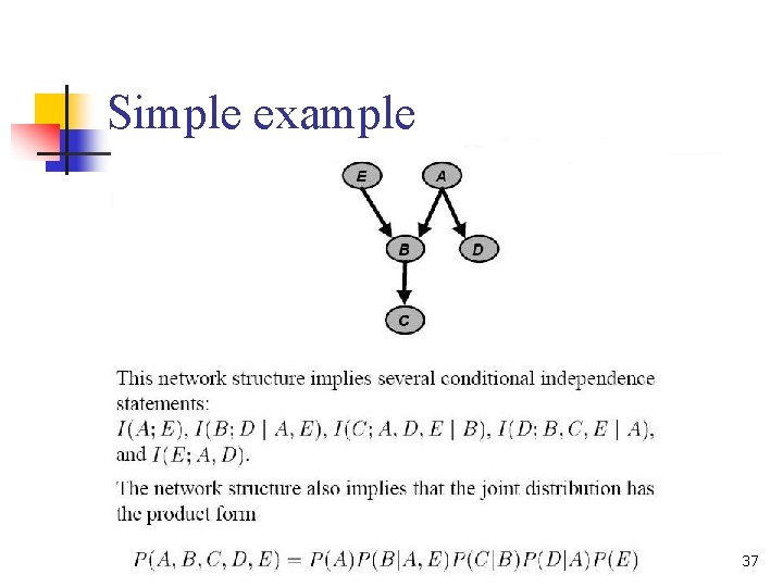
Simple example 37

Bayesian networks – properties n Encodes the Markov assumption : Each variable is independent of its non-descendants, given its parents in the graph n n n A graph-based model that captures properties of conditional independence between variables. Useful for describing processes composed of locally interacting components. Provide models of causal influence. 38

Equivalence classes n n Let Ind(G) be the set of independence statements (of the form X is independent of Y given Z). More than one graph can imply exactly the same set of independencies. Two graphs G’ and G’’ are equivalent if Ind(G’)=Ind(G’’), that is, both graphs are alternative ways of describing the same set of independencies. Equivalent graphs have the same underlying undirected graph but might disagree on the direction of some of the 39 arcs (we switch to PDAG).

Learning Bayesian Networks n n Given a training set D of independent instances of X, find a network B={G, θ} that best matches D. Several scoring functions are available. Finding the structure G that maximizes the score is a problem which is known to be NP-hard. For Heuristic search we need : n A score function which is decomposable For example - n S(G: D) = log P(D|G) + log P(G) + C An iterative search method For example - Greedy/stochastic hill climbing, simulated annealing… 40

Biological (causal) interpretation n n Edges: the parents of a variable are its immediate causes (the parent of a node is a transcription factor for this gene). A causal network models the effects of interventions: If X causes Y, then manipulating the value of X affects the value of Y, but not the other way around (If we knockout gene X then this will affect the expression of gene Y, but a knockout of gene Y has no effect on the expression of gene X). 41

Analyzing Expression Data n n n Random variable denote the expression level of individual genes. In addition, we can include random variables that denote other attributes that affect the system (experimental conditions, temporal indicators…). We want to learn one from the available data and use it to answer questions about the system. 42

Find high-scoring networks n n The data is not informative enough to determine which single model is the right one Focusing on features that are common to most of the possible models: n n Markov relation - indicates that two genes are related in some joint biological interaction or process (if there is either an edge between them, or both are parents of another variable (Pearl 1988)). Order relation - X is an ancestor of Y in all the networks of a given equivalence class (the given PDAG contain a directed path from X to Y). 43

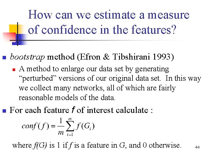
How can we estimate a measure of confidence in the features? n bootstrap method (Efron & Tibshirani 1993) n n A method to enlarge our data set by generating “perturbed” versions of our original data set. In this way we collect many networks, all of which are fairly reasonable models of the data. For each feature f of interest calculate : where f(G) is 1 if f is a feature in G, and 0 otherwise. 44

Local Probability Models In order to specify a Bayesian network model, we still need to choose the type of the local probability models we learn. In the current work, we consider two approaches: n n Multinomial model (discretizing to (-1, 0, 1). Linear Gaussian model. 45

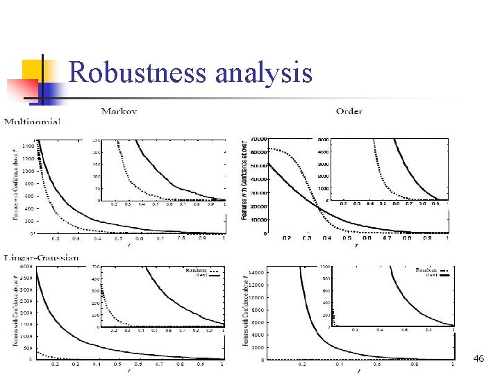
Robustness analysis 46

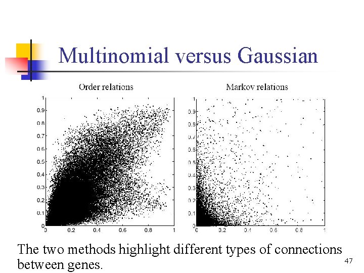
Multinomial versus Gaussian The two methods highlight different types of connections 47 between genes.

Biological Analysis n n n Order relations reveals existence of dominant genes. Out of all 800 genes only few seem to dominate the order (i. e. , appear before many genes). Top Markov relations reveals genes that most are functionally related. Nice presentation: http: //www. cs. huji. ac. il/~nirf/Gene. Expression/top 800/ 48

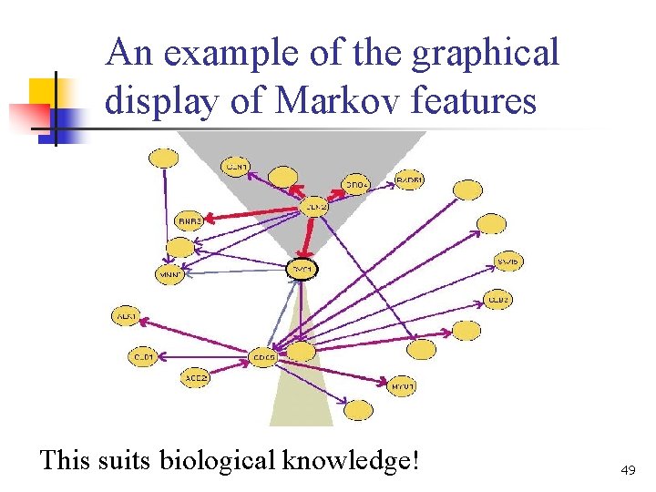
An example of the graphical display of Markov features This suits biological knowledge! 49

Application 2 summary n Using Bayesian networks to model genetic network: Ø ü § § Involves thousands of genes while current data sets contain a few dozen samples. This raises problems in computational complexity and the statistical significance of the results. Genetic regulation networks are sparse (gene assumed to have no more than a few dozen genes directly affect its transcription). Bayesian networks are especially suited for learning in such sparse domains. Did not use any (biological) prior knowledge. This theory can provide tools for experimental design. 50

Dynamic Bayesian Networks n n DBNs are an extension of Bayesian networks, which have been successfully applied to model expression data (Pe’er et al. , 2001). The main advantage that unlike BNs, DBNs allow for cycles, which are common in biological systems. In addition, DBNs can also improve our ability to learn causal relationships by relying on the temporal nature of the data. DBNs seem like a promising direction for modeling temporal system and recently a number of papers 51 discuss this model.

Application 3 [Holter 2000] Fundamental patterns underlying gene expression n n Algebraic approach. Using SVD to a model gene expression. 52

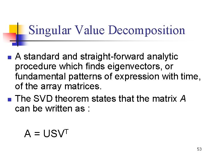
Singular Value Decomposition n n A standard and straight-forward analytic procedure which finds eigenvectors, or fundamental patterns of expression with time, of the array matrices. The SVD theorem states that the matrix A can be written as : A = USVT 53

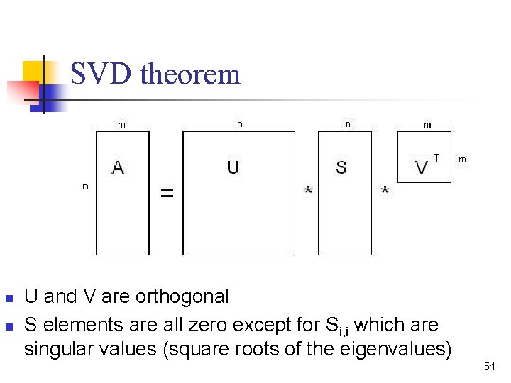
SVD theorem n n U and V are orthogonal S elements are all zero except for Si, i which are singular values (square roots of the eigenvalues) 54

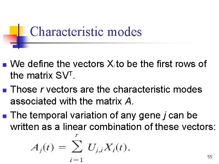
Characteristic modes n n n We define the vectors Xi to be the first rows of the matrix SVT. Those r vectors are the characteristic modes associated with the matrix A. The temporal variation of any gene j can be written as a linear combination of these vectors: 55

Results n n The first two values were significantly greater than the others for all three data sets, but the same is not true in a control calculation on random data. Only the first few modes are required to capture the essential features of the expression data in most cases (the modes reflect the genomewide expression pattern and are not genespecific). 56

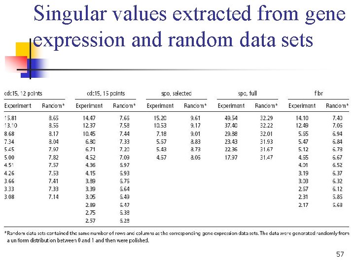
Singular values extracted from gene expression and random data sets 57

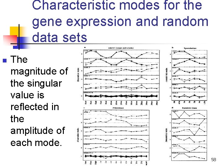
Characteristic modes for the gene expression and random data sets n The magnitude of the singular value is reflected in the amplitude of each mode. 58

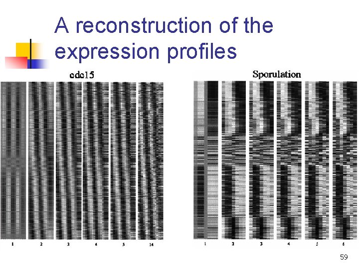
A reconstruction of the expression profiles 59

Analysis 1 n n n Type of ‘‘spectral’’ analysis : a gene expression profile can be precisely represented by specifying the magnitude and sign of the contribution of each of its characteristic modes. This suggests that at a gross level, most timedependent expression patterns are very simple. Data from SVD agree with previous knowledge 60 of expression patterns.

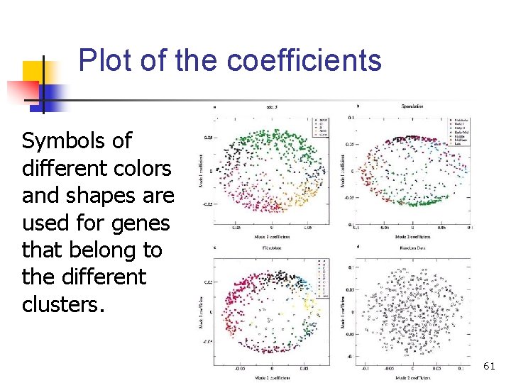
Plot of the coefficients Symbols of different colors and shapes are used for genes that belong to the different clusters. 61

Analysis 2 n n n The data points (which are not random) are concentrated near the perimeter of a circle or an ellipse, with the interior rather sparsely populated. Expression profiles clustered by more conventional methods correspond well to groups of genes with similar coefficients. Despite the evolutionary distance between yeast and humans, the observed behavior is both simple and similar. 62

Application 3 summary n n SVD has uncovered underlying patterns or ‘‘characteristic modes’’ in gene temporal profiles. The expression pattern of any particular gene can be represented precisely by a linear combination of the modes with gene-specific coefficients. A good approximation of the exact pattern can be obtained by using just a few of the modes, underscoring the simplicity of the gene expression patterns. This paradigm may find expression patterns that would not be detected using other methods. 63

Application 3 b [Holter et al 2001] Dynamic modeling n n n In the previous application we treated the gene expression pattern as a ‘‘static’’ image and derived the underlying genomewide characteristic modes of which it is composed. Now we carry out a dynamical analysis, exploring the possible causal relationships among the genes by deducing a time translation matrix for the characteristic modes defined by SVD. This matrix predicts future expression levels of genes based on their expression levels at some initial time. 64

How to deduce a time translation matrix? n n n To uniquely and unambiguously determine the g 2 elements of the matrix, one needs a set of g 2 linearly independent equations. D’haeseleer [1999] used a nonlinear interpolation scheme to guess the shapes of gene expression profiles between the measured time points (speculative). Van Someren [2000] chose to cluster the genes and study the interrelationships between the clusters (based on profile similarity). 65

Deduce a time translation matrix by using SVD n n n The SVD construction gives a linear combination of which exactly describes the expression pattern of each gene. The modes form a linearly independent basis set. The problem is mathematically well defined and tractable if one considers the causal relationships among the modes. 66

Analysis n n The causal links between the modes, and thence the genes, involve just a few essential connections. Any additional connections among the genes must therefore provide redundancy in the network. An important corollary is that it may be impossible to determine detailed connectivities among genes with just the micro-array data, because the number of genes greatly exceeds the number of contributing modes. 67

Application 3 b summary n n n A model in which the expression levels of the genes at a given time are linear combinations of their levels at a previous time. Temporal evolution of the gene expression profiles can be described by using a ‘‘time translation’’ matrix, which reflects the magnitude of the connectivities between genes. Because there are only a few essential connections among modes and therefore among genes, additional links provide redundancy in the network. 68

References §Yaacov Lindzen’s presentation “Introduction to Micro-arrays” §“Genetic network analysis in light of massively parallel biological data acquisition”. Szallasi, 1999, PSB §“Exploring the metabolic and genetic control of gene expression on a genomic scale”. De. Risi et al, 1997, Science §“Using Bayesian networks to analyze expression data”. Friedman et al, 2000. §“Fundamental patterns underlying gene expression profiles: Simplicity from complexity”. Holter et al, 2000, Genetics §“Dynamic modeling of gene expression data”. Holter et al, 2001, Genetics §“Analyzing time series gene expression data”. Bar Joseph, 69 2004, Bioinformatics