Overview of Kernel Methods Steve Vincent Adapted from

Overview of Kernel Methods Steve Vincent Adapted from John Shawe-Taylor and Nello Christianini, Kernel Methods for Pattern Analysis

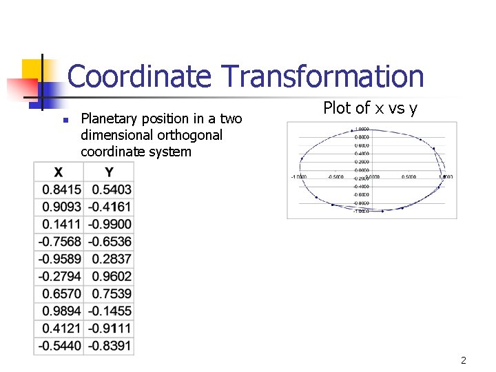
Coordinate Transformation n Planetary position in a two dimensional orthogonal coordinate system Plot of x vs y 2

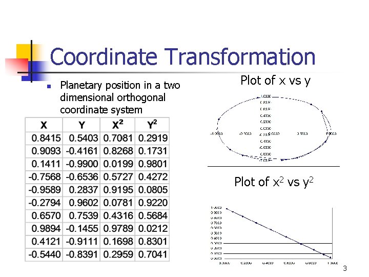
Coordinate Transformation n Planetary position in a two dimensional orthogonal coordinate system Plot of x vs y Plot of x 2 vs y 2 3

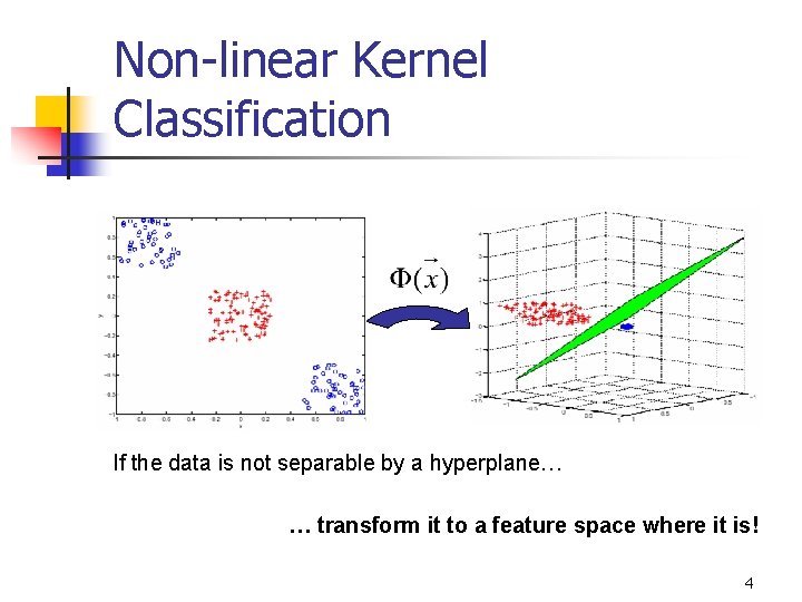
Non-linear Kernel Classification If the data is not separable by a hyperplane… … transform it to a feature space where it is! 4

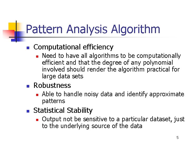
Pattern Analysis Algorithm n Computational efficiency n n Robustness n n Need to have all algorithms to be computationally efficient and that the degree of any polynomial involved should render the algorithm practical for large data sets Able to handle noisy data and identify approximate patterns Statistical Stability n Output not be sensitive to a particular dataset, just to the underlying source of the data 5

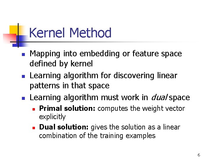
Kernel Method n n n Mapping into embedding or feature space defined by kernel Learning algorithm for discovering linear patterns in that space Learning algorithm must work in dual space n n Primal solution: computes the weight vector explicitly Dual solution: gives the solution as a linear combination of the training examples 6

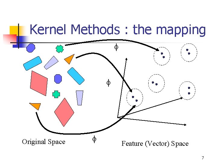
Kernel Methods : the mapping Original Space Feature (Vector) Space 7

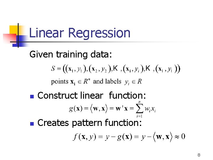
Linear Regression Given training data: n Construct linear function: n Creates pattern function: 8

1 -d Regression 9

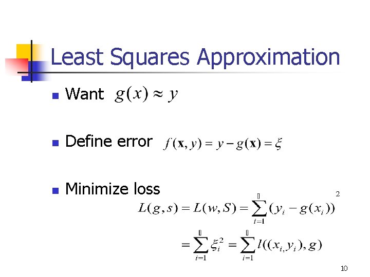
Least Squares Approximation n Want n Define error n Minimize loss 10

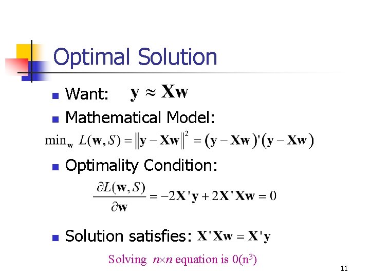
Optimal Solution n Want: Mathematical Model: n Optimality Condition: n Solution satisfies: n Solving n n equation is 0(n 3) 11

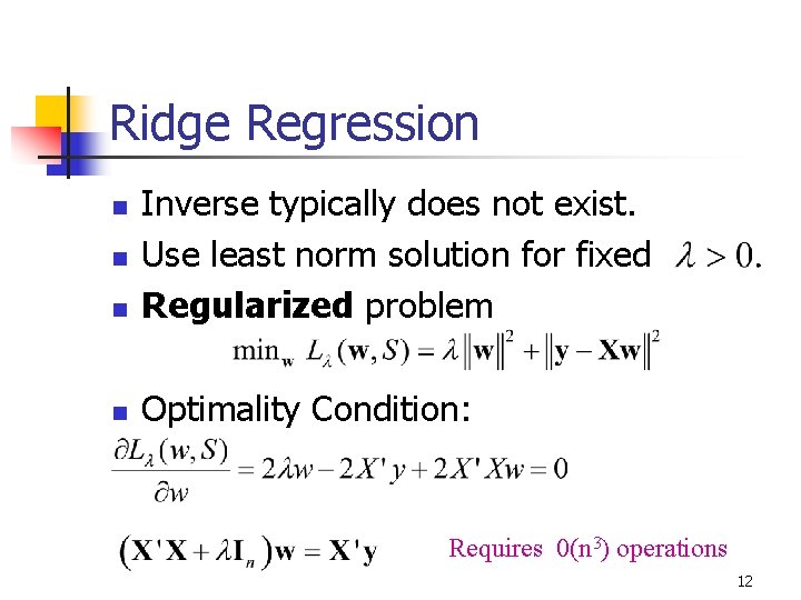
Ridge Regression n Inverse typically does not exist. Use least norm solution for fixed Regularized problem n Optimality Condition: n n Requires 0(n 3) operations 12

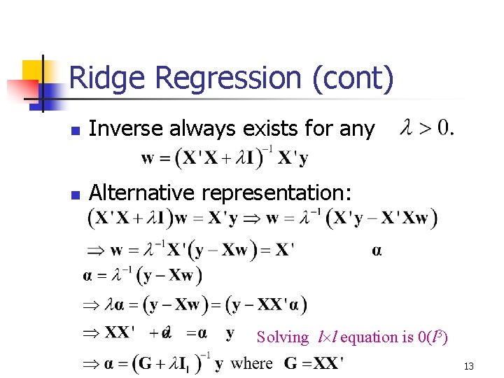
Ridge Regression (cont) n Inverse always exists for any n Alternative representation: Solving l l equation is 0(l 3) 13

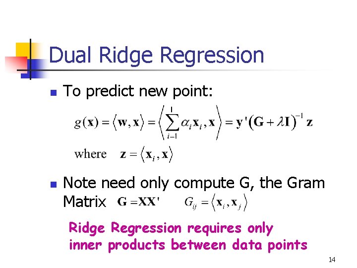
Dual Ridge Regression n n To predict new point: Note need only compute G, the Gram Matrix Ridge Regression requires only inner products between data points 14

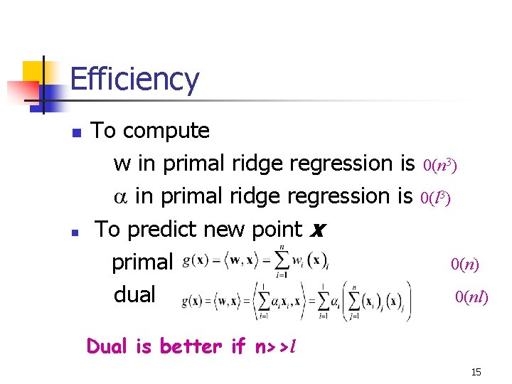
Efficiency n n To compute w in primal ridge regression is 0(n 3) in primal ridge regression is 0(l 3) To predict new point x primal 0(n) dual 0(nl) Dual is better if n>>l 15

Notes on Ridge Regression n n “Regularization” is key to address stability and regularization. Regularization lets method work when n>>l. Dual more efficient when n>>l. Dual only requires inner products of data. 16

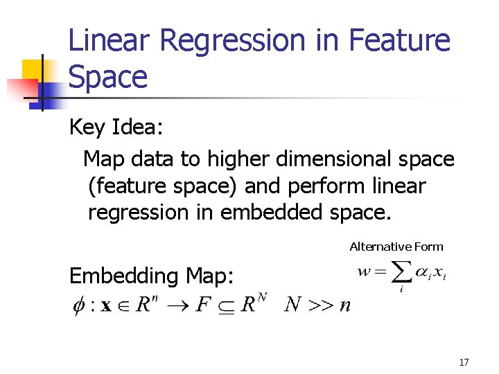
Linear Regression in Feature Space Key Idea: Map data to higher dimensional space (feature space) and perform linear regression in embedded space. Alternative Form Embedding Map: 17

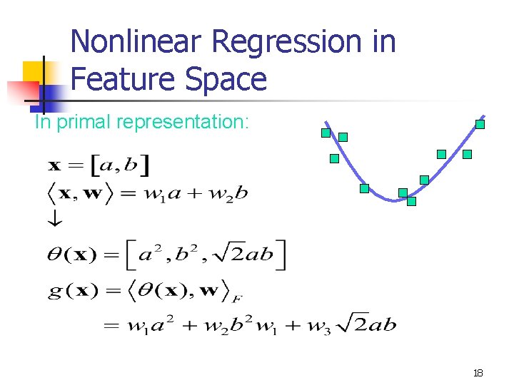
Nonlinear Regression in Feature Space In primal representation: 18

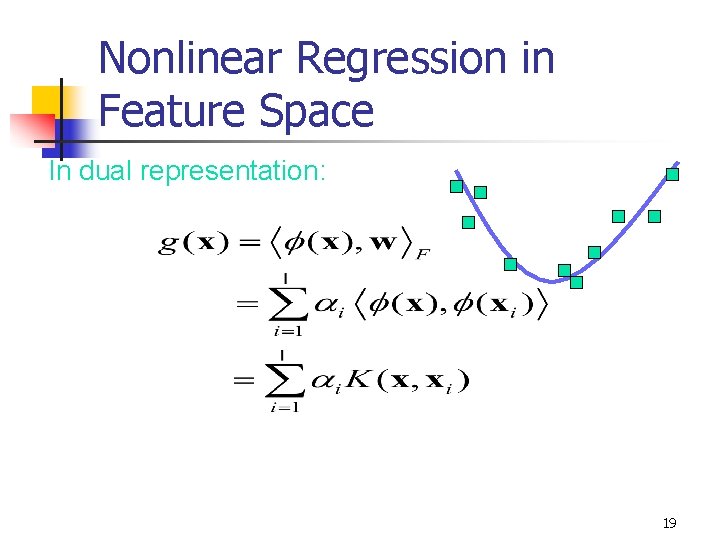
Nonlinear Regression in Feature Space In dual representation: 19

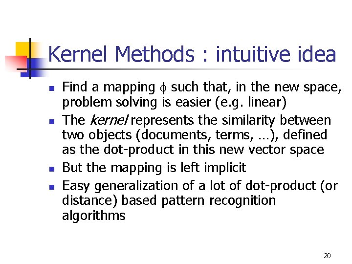
Kernel Methods : intuitive idea n n Find a mapping such that, in the new space, problem solving is easier (e. g. linear) The kernel represents the similarity between two objects (documents, terms, …), defined as the dot-product in this new vector space But the mapping is left implicit Easy generalization of a lot of dot-product (or distance) based pattern recognition algorithms 20

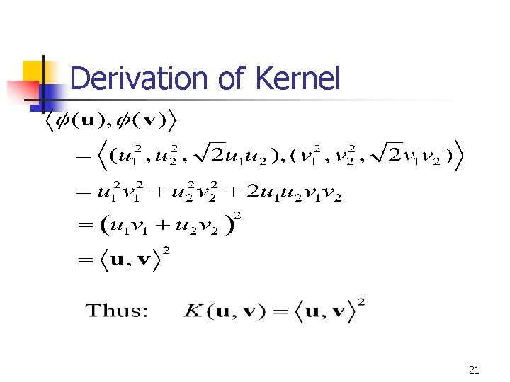
Derivation of Kernel 21

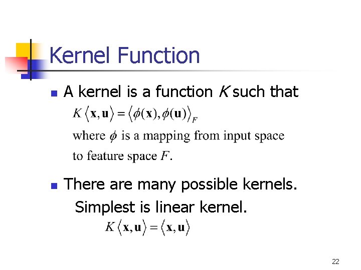
Kernel Function n n A kernel is a function K such that There are many possible kernels. Simplest is linear kernel. 22

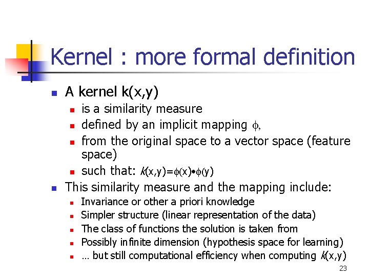
Kernel : more formal definition n A kernel k(x, y) n is a similarity measure n defined by an implicit mapping , n from the original space to a vector space (feature space) n such that: k(x, y)= (x) • (y) This similarity measure and the mapping include: n n n Invariance or other a priori knowledge Simpler structure (linear representation of the data) The class of functions the solution is taken from Possibly infinite dimension (hypothesis space for learning) … but still computational efficiency when computing k(x, y) 23

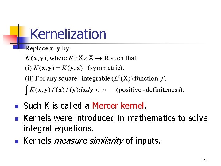
Kernelization n Such K is called a Mercer kernel. Kernels were introduced in mathematics to solve integral equations. Kernels measure similarity of inputs. 24

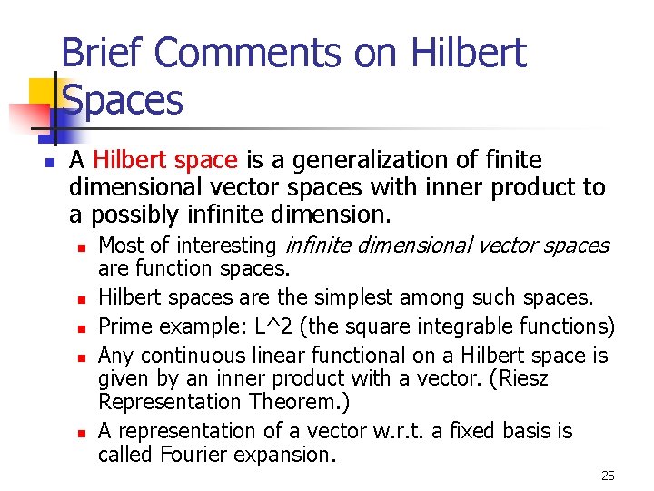
Brief Comments on Hilbert Spaces n A Hilbert space is a generalization of finite dimensional vector spaces with inner product to a possibly infinite dimension. n n n Most of interesting infinite dimensional vector spaces are function spaces. Hilbert spaces are the simplest among such spaces. Prime example: L^2 (the square integrable functions) Any continuous linear functional on a Hilbert space is given by an inner product with a vector. (Riesz Representation Theorem. ) A representation of a vector w. r. t. a fixed basis is called Fourier expansion. 25

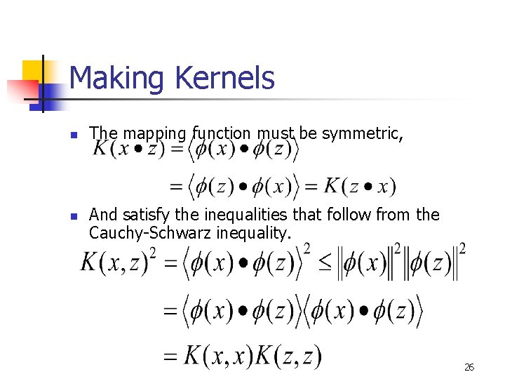
Making Kernels n n The mapping function must be symmetric, And satisfy the inequalities that follow from the Cauchy-Schwarz inequality. 26

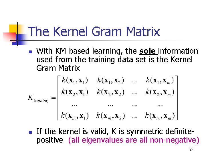
The Kernel Gram Matrix n n With KM-based learning, the sole information used from the training data set is the Kernel Gram Matrix If the kernel is valid, K is symmetric definitepositive (all eigenvalues are all non-negative) 27

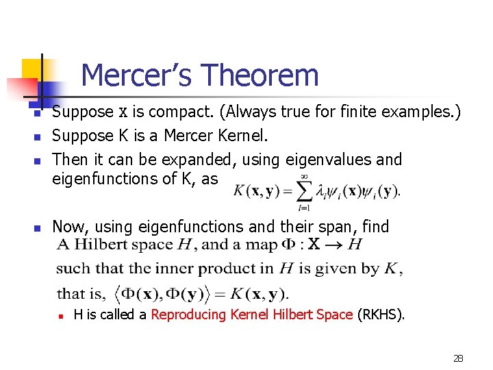
Mercer’s Theorem n n Suppose X is compact. (Always true for finite examples. ) Suppose K is a Mercer Kernel. Then it can be expanded, using eigenvalues and eigenfunctions of K, as Now, using eigenfunctions and their span, find n H is called a Reproducing Kernel Hilbert Space (RKHS). 28

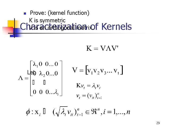
n Prove: (kernel function) K is symmetric V is an orthogonal matrix. Characterization of Kernels Let 29

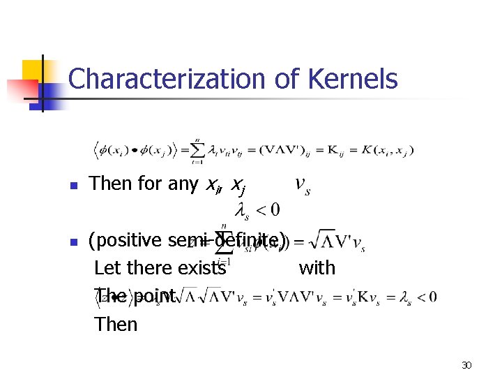
Characterization of Kernels n n Then for any xi, xj (positive semi-definite) Let there exists with The point Then 30

Reproducing Kernel Hilbert Spaces n n Reproducing Kernel Hilbert Spaces (RKHS) [1] The Hilbert space L 2 is too “big” for our purpose, containing too many non-smooth functions. One approach to obtaining restricted, smooth spaces is the RKHS approach. A RKHS is “smaller” then a general Hilbert space. Define the reproducing kernel map (to each x we associate a function k(. , x)) 31

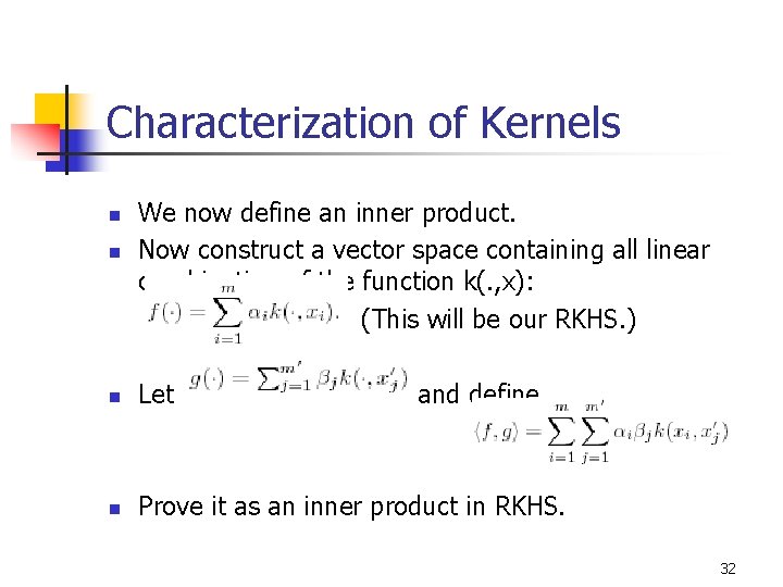
Characterization of Kernels n n We now define an inner product. Now construct a vector space containing all linear combination of the function k(. , x): (This will be our RKHS. ) n Let and define n Prove it as an inner product in RKHS. 32

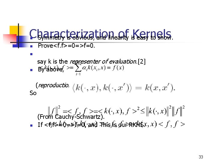
Characterization of is. Kernels Symmetry is obvious, and linearity easy to show. n n Prove<f. f>=0=>f=0. n n say k is the representer of evaluation. [2] By above, (reproduction property) So n (From Cauchy-Schwartz). If <f, f>=0=>f=0, and This is our RKHS. 33

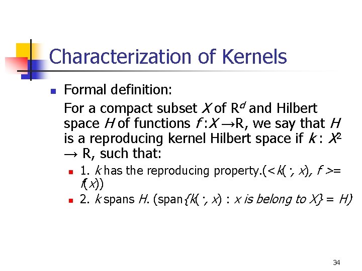
Characterization of Kernels n Formal definition: For a compact subset X of Rd and Hilbert space H of functions f : X →R, we say that H is a reproducing kernel Hilbert space if k : X 2 → R, such that: n n 1. k has the reproducing property. (<k(·, x), f >= f(x)) 2. k spans H. (span{k(·, x) : x is belong to X} = H) 34

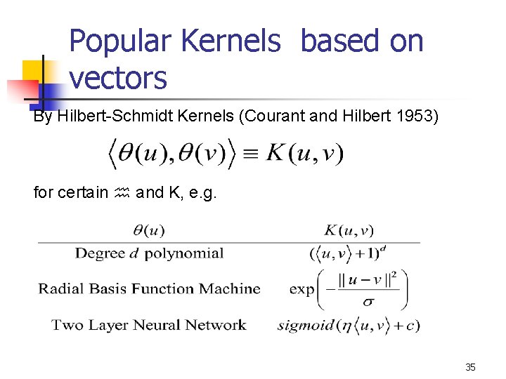
Popular Kernels based on vectors By Hilbert-Schmidt Kernels (Courant and Hilbert 1953) for certain and K, e. g. 35

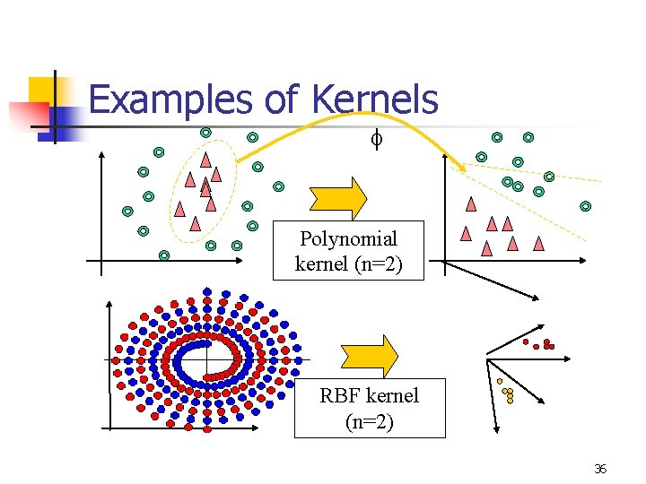
Examples of Kernels Polynomial kernel (n=2) RBF kernel (n=2) 36

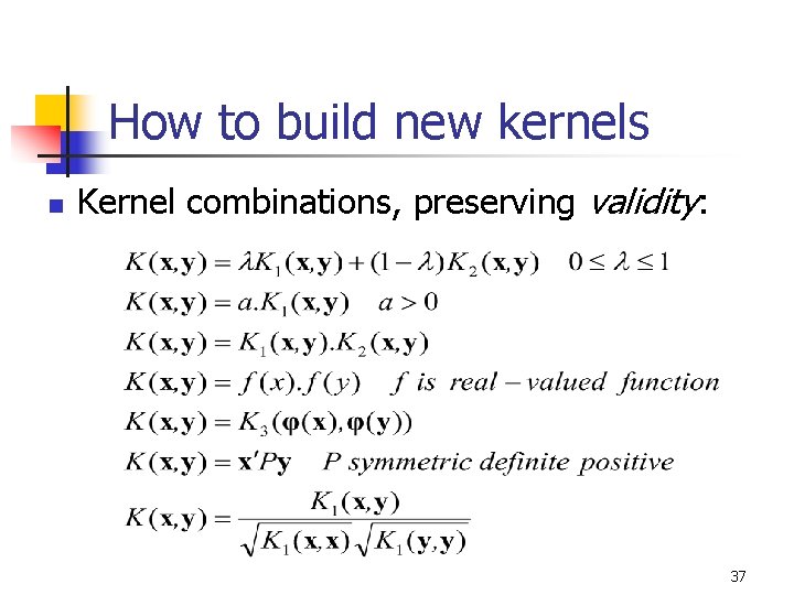
How to build new kernels n Kernel combinations, preserving validity: 37

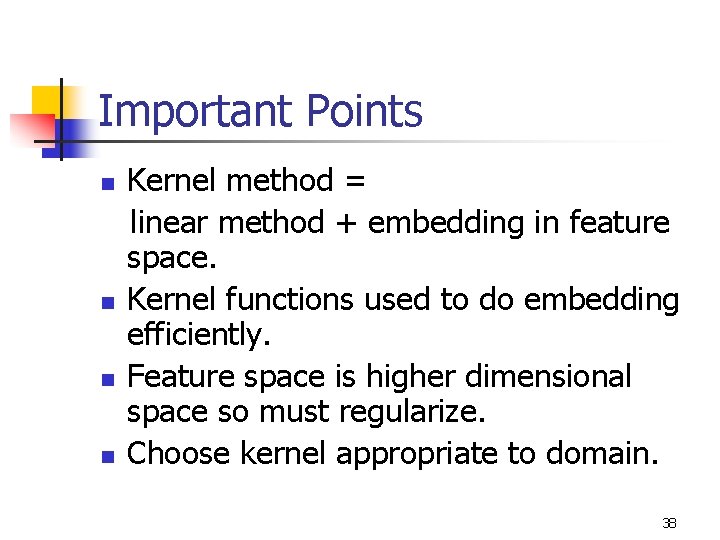
Important Points n n Kernel method = linear method + embedding in feature space. Kernel functions used to do embedding efficiently. Feature space is higher dimensional space so must regularize. Choose kernel appropriate to domain. 38

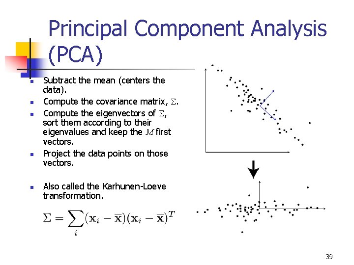
Principal Component Analysis (PCA) n n n Subtract the mean (centers the data). Compute the covariance matrix, S. Compute the eigenvectors of S, sort them according to their eigenvalues and keep the M first vectors. Project the data points on those vectors. Also called the Karhunen-Loeve transformation. 39

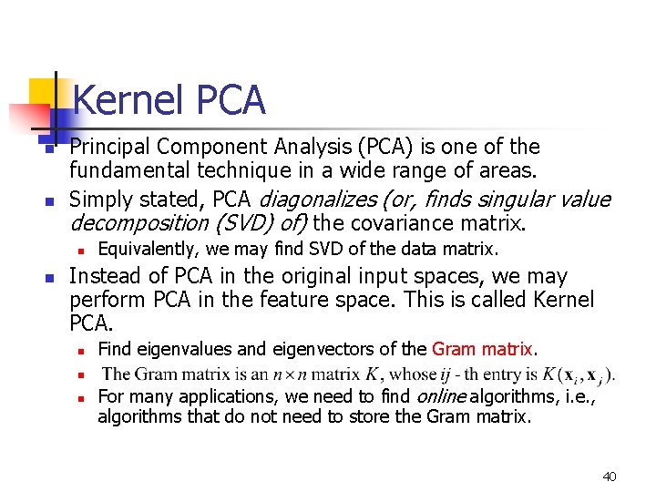
Kernel PCA n n Principal Component Analysis (PCA) is one of the fundamental technique in a wide range of areas. Simply stated, PCA diagonalizes (or, finds singular value decomposition (SVD) of) the covariance matrix. n n Equivalently, we may find SVD of the data matrix. Instead of PCA in the original input spaces, we may perform PCA in the feature space. This is called Kernel PCA. n Find eigenvalues and eigenvectors of the Gram matrix. n n For many applications, we need to find online algorithms, i. e. , algorithms that do not need to store the Gram matrix. 40

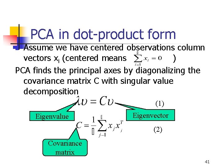
PCA in dot-product form Assume we have centered observations column vectors xi (centered means ) PCA finds the principal axes by diagonalizing the covariance matrix C with singular value decomposition n (1) Eigenvalue Eigenvector (2) Covariance matrix 41

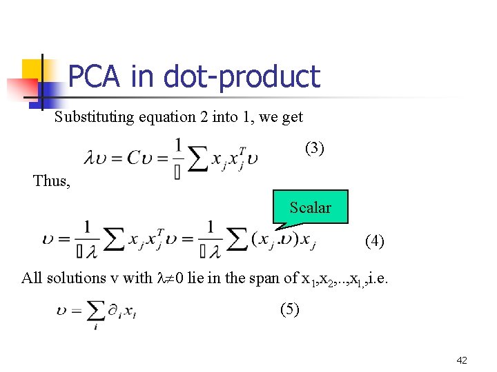
PCA in dot-product Substituting equation 2 into 1, we get (3) Thus, Scalar (4) All solutions v with 0 lie in the span of x 1, x 2, . . , xl, , i. e. (5) 42

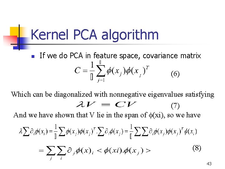
Kernel PCA algorithm n If we do PCA in feature space, covariance matrix (6) Which can be diagonalized with nonnegative eigenvalues satisfying (7) And we have shown that V lie in the span of (xi), so we have (8) 43

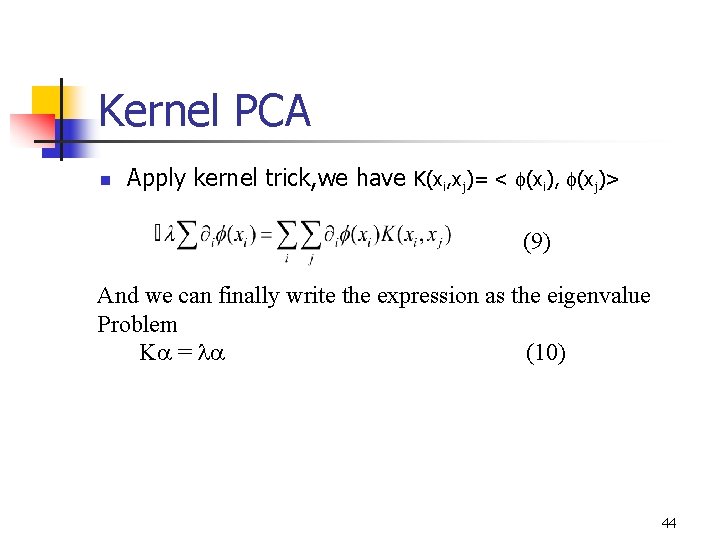
Kernel PCA n Apply kernel trick, we have K(xi, xj)= < (xi), (xj)> (9) And we can finally write the expression as the eigenvalue Problem K = (10) 44

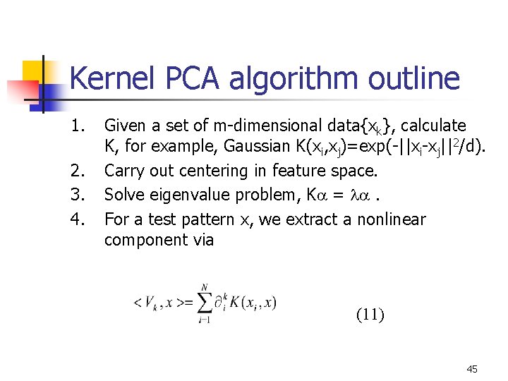
Kernel PCA algorithm outline 1. 2. 3. 4. Given a set of m-dimensional data{xk}, calculate K, for example, Gaussian K(xi, xj)=exp(-||xi-xj||2/d). Carry out centering in feature space. Solve eigenvalue problem, K = . For a test pattern x, we extract a nonlinear component via (11) 45

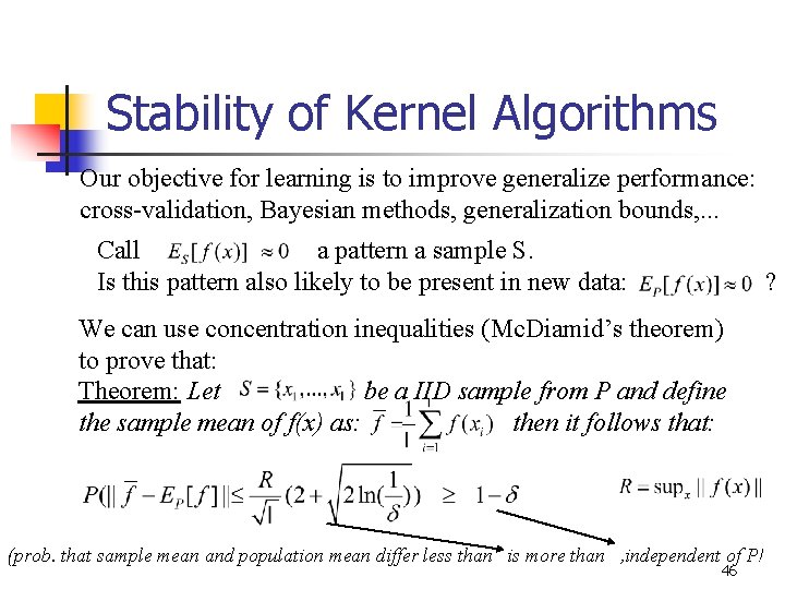
Stability of Kernel Algorithms Our objective for learning is to improve generalize performance: cross-validation, Bayesian methods, generalization bounds, . . . Call a pattern a sample S. Is this pattern also likely to be present in new data: ? We can use concentration inequalities (Mc. Diamid’s theorem) to prove that: Theorem: Let be a IID sample from P and define the sample mean of f(x) as: then it follows that: (prob. that sample mean and population mean differ less than is more than , independent of P! 46

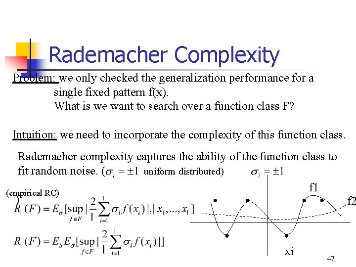
Rademacher Complexity Problem: we only checked the generalization performance for a single fixed pattern f(x). What is we want to search over a function class F? Intuition: we need to incorporate the complexity of this function class. Rademacher complexity captures the ability of the function class to fit random noise. ( uniform distributed) f 1 (empirical RC) xi 47 f 2

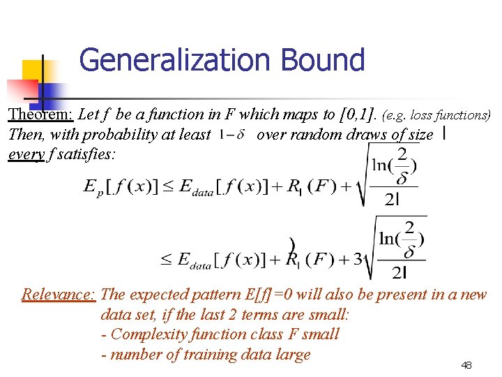
Generalization Bound Theorem: Let f be a function in F which maps to [0, 1]. (e. g. loss functions) Then, with probability at least over random draws of size every f satisfies: Relevance: The expected pattern E[f]=0 will also be present in a new data set, if the last 2 terms are small: - Complexity function class F small - number of training data large 48

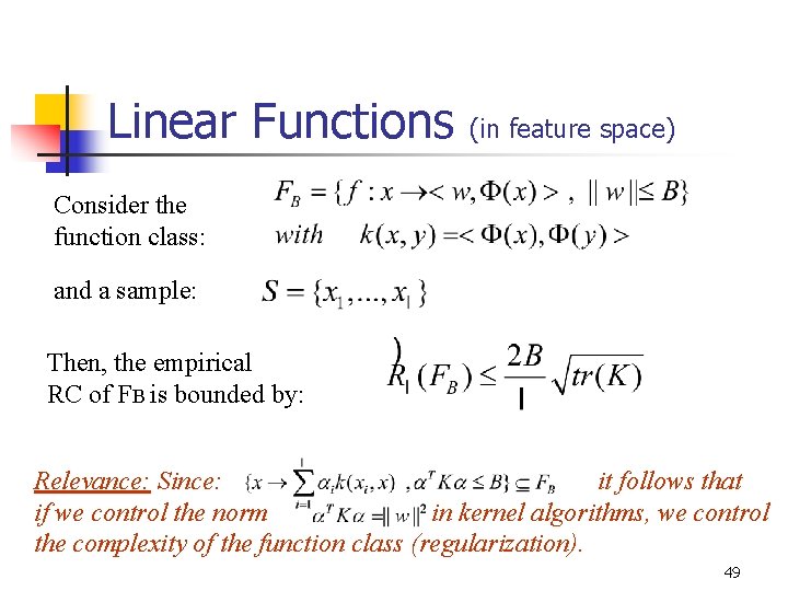
Linear Functions (in feature space) Consider the function class: and a sample: Then, the empirical RC of FB is bounded by: Relevance: Since: it follows that if we control the norm in kernel algorithms, we control the complexity of the function class (regularization). 49

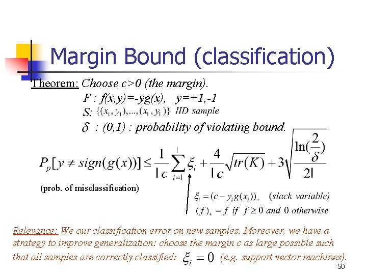
Margin Bound (classification) Theorem: Choose c>0 (the margin). F : f(x, y)=-yg(x), y=+1, -1 S: : (0, 1) : probability of violating bound. (prob. of misclassification) Relevance: We our classification error on new samples. Moreover, we have a strategy to improve generalization: choose the margin c as large possible such that all samples are correctly classified: (e. g. support vector machines). 50

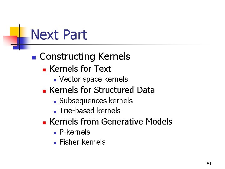
Next Part n Constructing Kernels n Kernels for Text n n Kernels for Structured Data n n n Vector space kernels Subsequences kernels Trie-based kernels Kernels from Generative Models n n P-kernels Fisher kernels 51