Overview n representing region in 2 ways n

Overview n representing region in 2 ways n n n in terms of its external characteristics (its boundary) focus on shape characteristics in terms of its internal characteristics (its region) focus on regional properties, e. g. , color, texture sometimes, we may need to use both ways 1

Overview n n Description describes the region based on the chosen representation ex. n n representation boundary description length of the boundary, orientation of the straight line joining its extreme points, and the number of concavities in the boundary. 2

Sensitivity n feature selected as descriptors should be as insensitive as possible to variations in n n size translation rotation following descriptors satisfy one or more of these properties. 3

Representation n Segmentation techniques yield raw data in the form of pixels along a boundary or pixels contained in a region these data sometimes are used directly to obtain descriptors standard uses techniques to compute more useful data (descriptors) from the raw data in order to decrease the size of data. 4

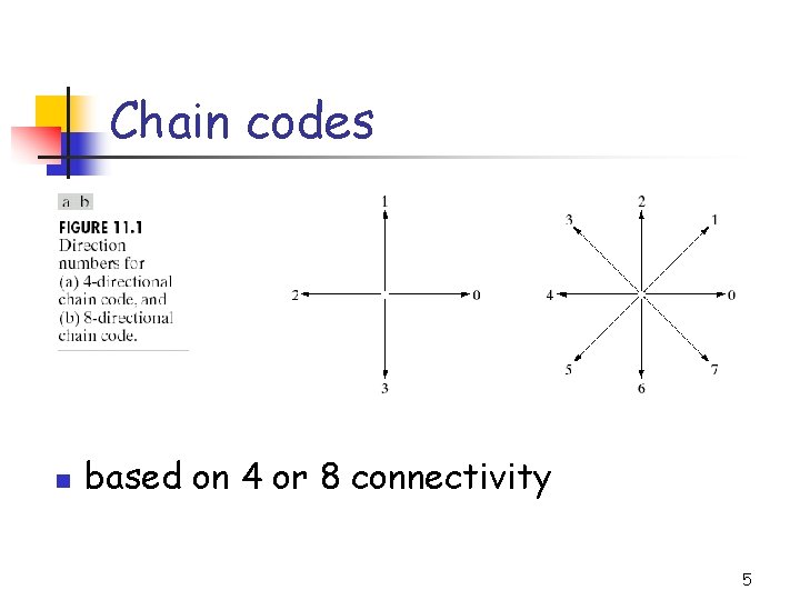
Chain codes n based on 4 or 8 connectivity 5

6

Chain codes n unacceptable because n n the resulting chain of codes tends to be quite long any small disturbances along the boundary due to noise or imperfect segmentation cause changes in the code that may not be related to the shape of the boundary 7

Chain codes n circumvent the problems by n n resample the boundary by selecting a larger grid spacing however, different grid can generate different chain codes starting point is arbitrary need to normalize the generated code so that codes with different starting point will become the same. 8

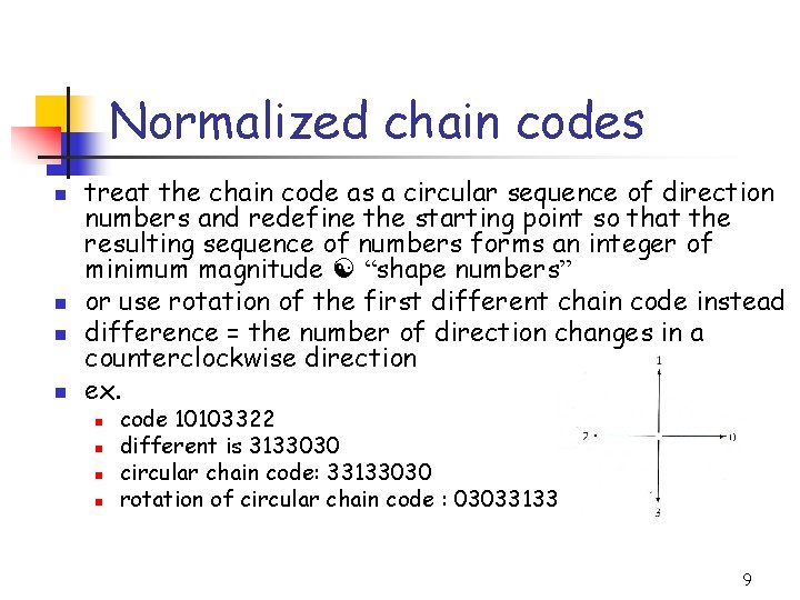
Normalized chain codes n n treat the chain code as a circular sequence of direction numbers and redefine the starting point so that the resulting sequence of numbers forms an integer of minimum magnitude “shape numbers” or use rotation of the first different chain code instead difference = the number of direction changes in a counterclockwise direction ex. n n code 10103322 different is 3133030 circular chain code: 33133030 rotation of circular chain code : 03033133 9

Normalized chain codes n n are exact only if the boundaries are invariant to rotation and scale change. but these are seldom cases. 10

Polygonal Approximations n n n boundary can be approximated with arbitrary accuracy by a polygon try to capture the “essence” of the boundary shape with the fewest possible polygonal segments. not trivial and time consuming 11

Minimum perimeter polygons n n n if each cell encompass only one point on the boundary error is at most be d is the minimum possible distance between different pixels 12

Merging techniques n n based on average error or other criteria merge points along the boundary until the least square error line fit of the points merged so far exceeds a preset threshold 13

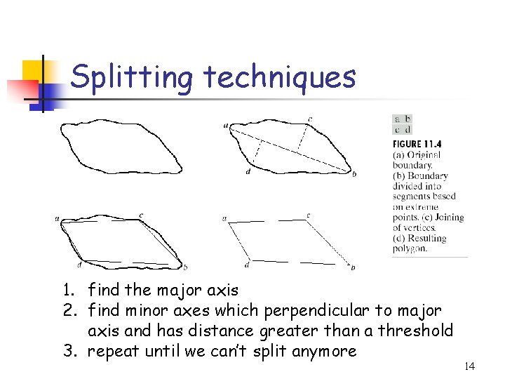
Splitting techniques 1. find the major axis 2. find minor axes which perpendicular to major axis and has distance greater than a threshold 3. repeat until we can’t split anymore 14

Signatures map 2 D function to 1 D function 15

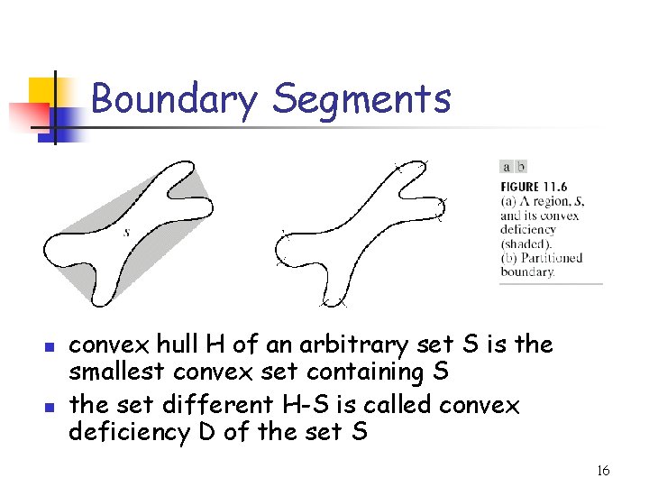
Boundary Segments n n convex hull H of an arbitrary set S is the smallest convex set containing S the set different H-S is called convex deficiency D of the set S 16

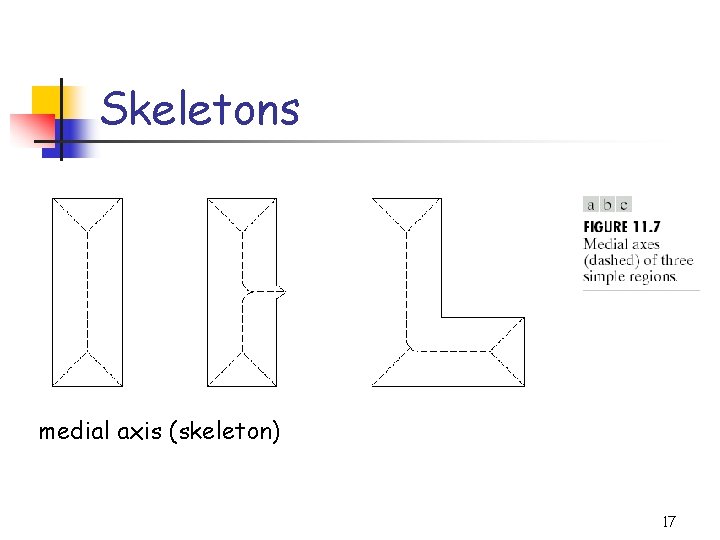
Skeletons medial axis (skeleton) 17

MAT n MAT of region R with border B is as follows. n n n for each point p in R, we find its closest neighbor in B. if p has more than one such neighbor, it is said to belong to the medial axis of R closest depends on the definition of a distance 18

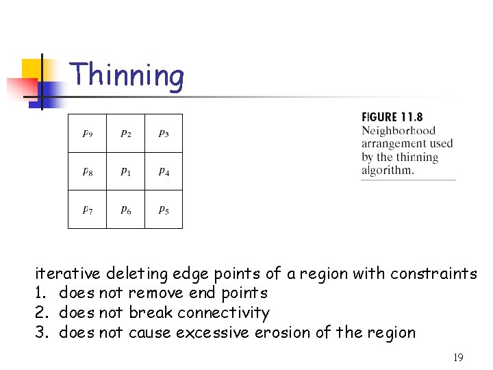
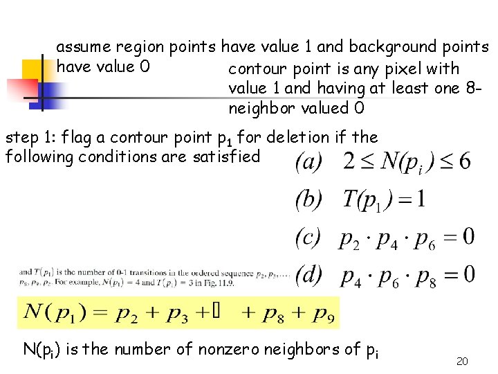
Thinning iterative deleting edge points of a region with constraints 1. does not remove end points 2. does not break connectivity 3. does not cause excessive erosion of the region 19

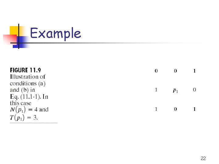
assume region points have value 1 and background points have value 0 contour point is any pixel with value 1 and having at least one 8 neighbor valued 0 step 1: flag a contour point p 1 for deletion if the following conditions are satisfied N(pi) is the number of nonzero neighbors of pi 20

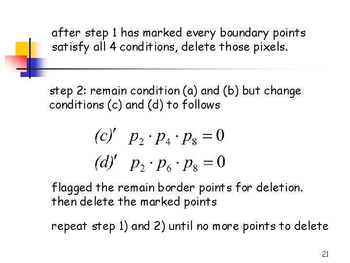
after step 1 has marked every boundary points satisfy all 4 conditions, delete those pixels. step 2: remain condition (a) and (b) but change conditions (c) and (d) to follows flagged the remain border points for deletion. then delete the marked points repeat step 1) and 2) until no more points to delete 21

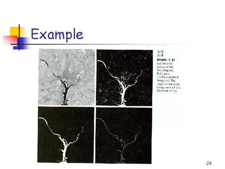
Example 22

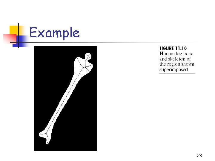
Example 23

Example 24

Boundary Descriptors n n n length of a boundary diameters Eccentricity shape numbers Fourier descriptors 25

Length of a boundary n n the number of pixels along a boundary give a rough approximation of its length 26

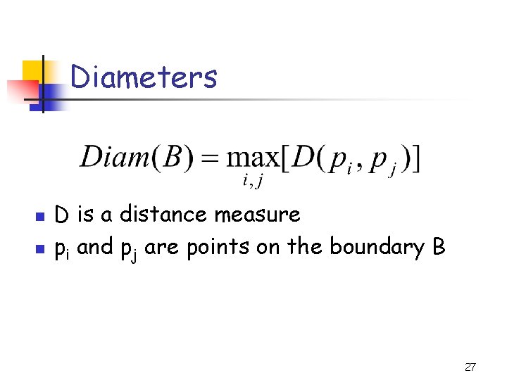
Diameters n n D is a distance measure pi and pj are points on the boundary B 27

Eccentricity n n n ratio of the major to the minor axis major axis = the line connecting the two extreme points that comprise the diameter minor axis = the line perpendicular to the major axis 28

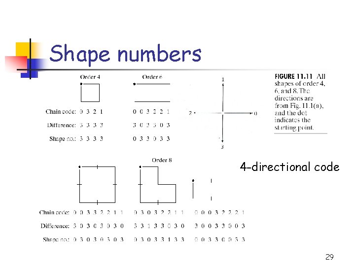
Shape numbers 4 -directional code 29

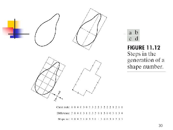
30

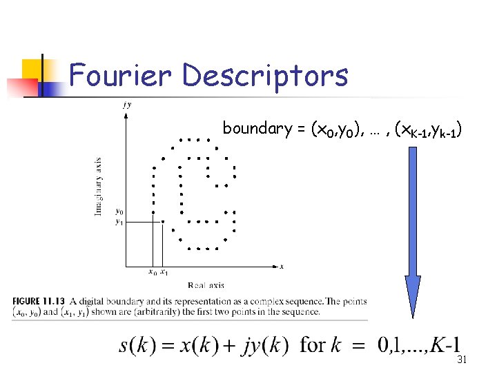
Fourier Descriptors boundary = (x 0, y 0), … , (x. K-1, yk-1) 31

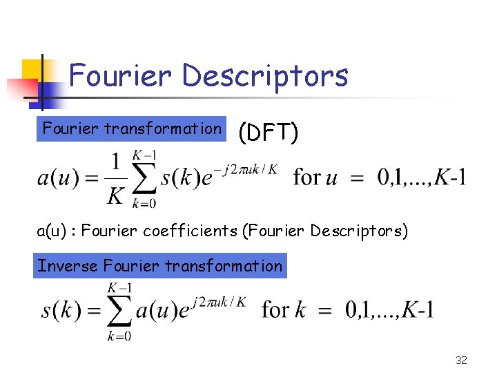
Fourier Descriptors Fourier transformation (DFT) a(u) : Fourier coefficients (Fourier Descriptors) Inverse Fourier transformation 32

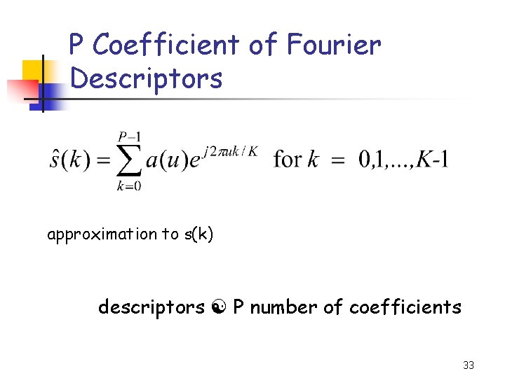
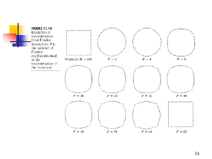
P Coefficient of Fourier Descriptors approximation to s(k) descriptors P number of coefficients 33

34

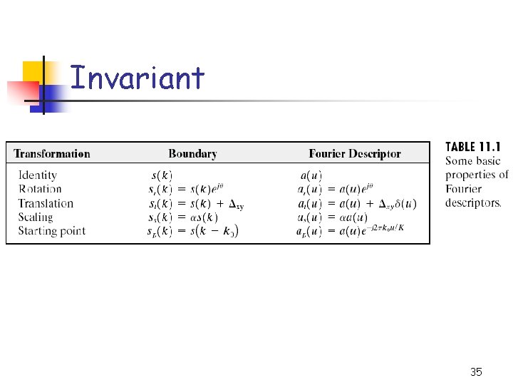
Invariant 35

Regional Descriptors n n n area perimeter compactness topological descriptors texture 36

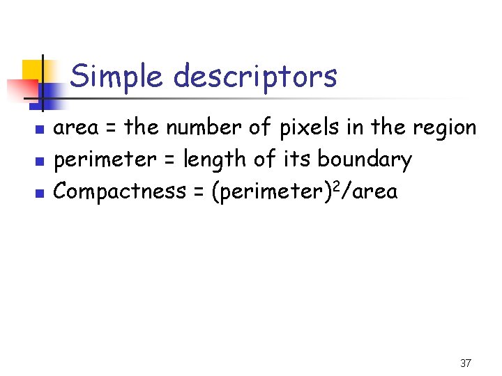
Simple descriptors n n n area = the number of pixels in the region perimeter = length of its boundary Compactness = (perimeter)2/area 37

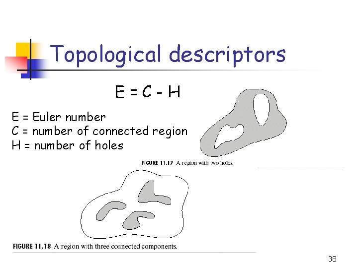
Topological descriptors E=C-H E = Euler number C = number of connected region H = number of holes 38

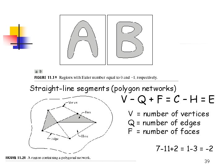
Straight-line segments (polygon networks) V–Q+F=C–H=E V = number of vertices Q = number of edges F = number of faces 7 -11+2 = 1 -3 = -2 39

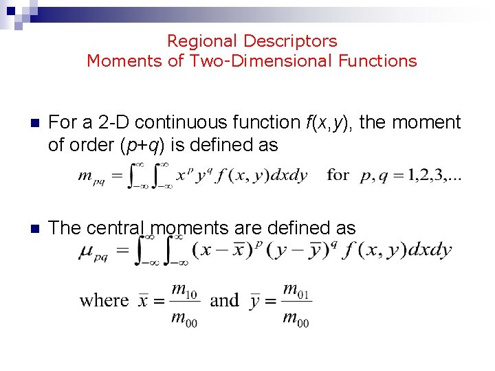
Regional Descriptors Moments of Two-Dimensional Functions n For a 2 -D continuous function f(x, y), the moment of order (p+q) is defined as n The central moments are defined as

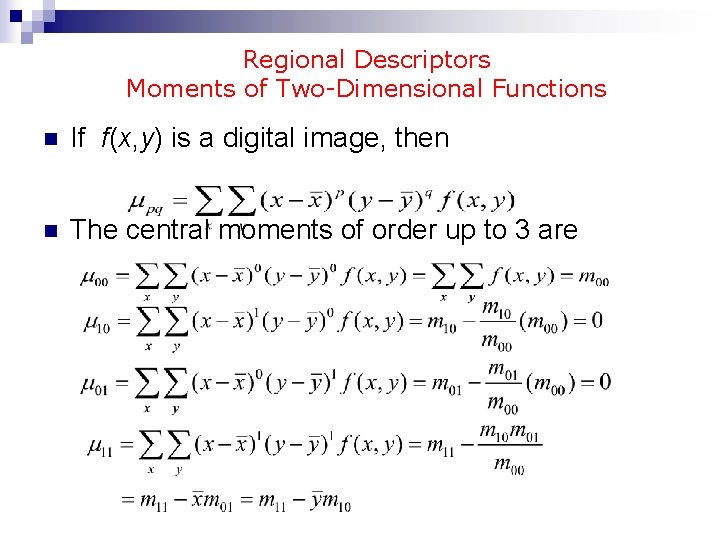
Regional Descriptors Moments of Two-Dimensional Functions n If f(x, y) is a digital image, then n The central moments of order up to 3 are

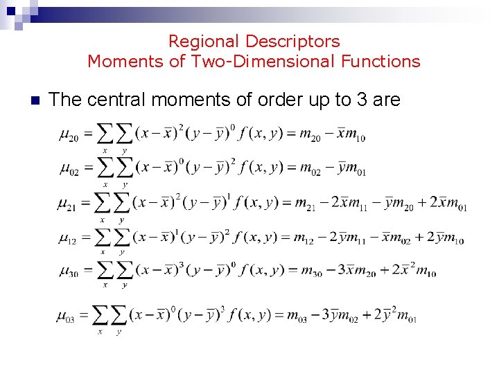
Regional Descriptors Moments of Two-Dimensional Functions n The central moments of order up to 3 are

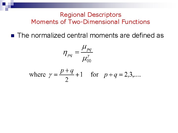
Regional Descriptors Moments of Two-Dimensional Functions n The normalized central moments are defined as

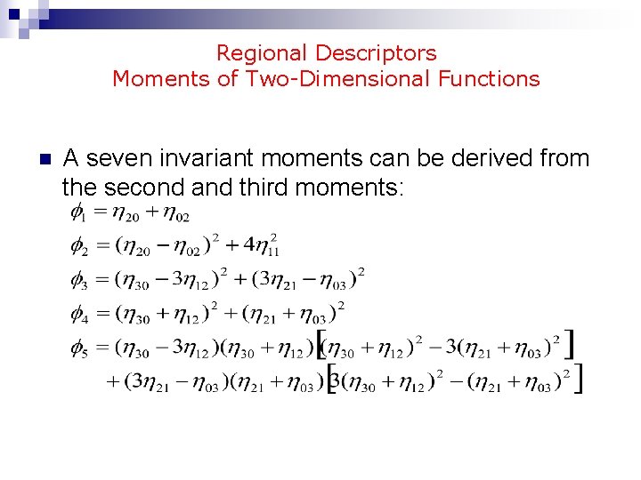
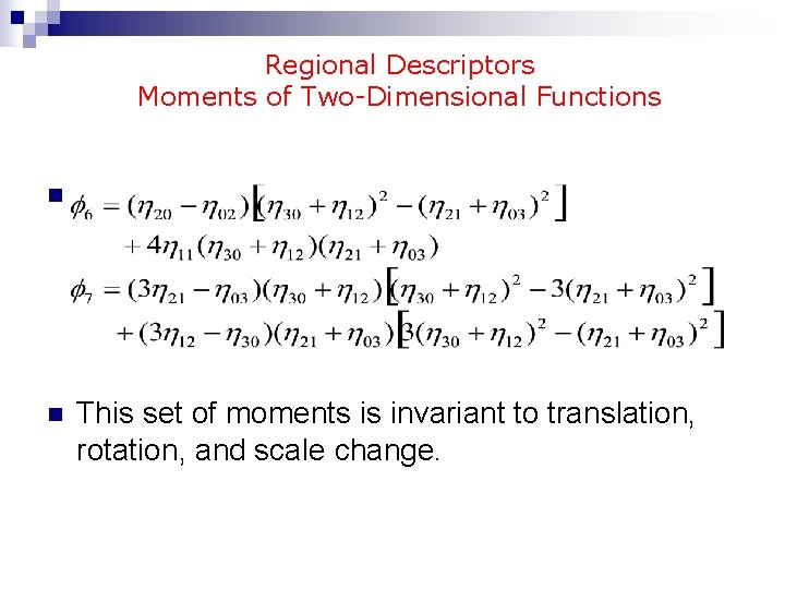
Regional Descriptors Moments of Two-Dimensional Functions n A seven invariant moments can be derived from the second and third moments:

Regional Descriptors Moments of Two-Dimensional Functions n n This set of moments is invariant to translation, rotation, and scale change.

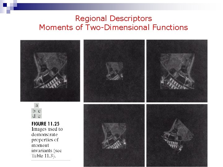
Regional Descriptors Moments of Two-Dimensional Functions

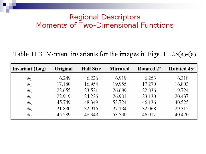
Regional Descriptors Moments of Two-Dimensional Functions Table 11. 3 Moment invariants for the images in Figs. 11. 25(a)-(e).

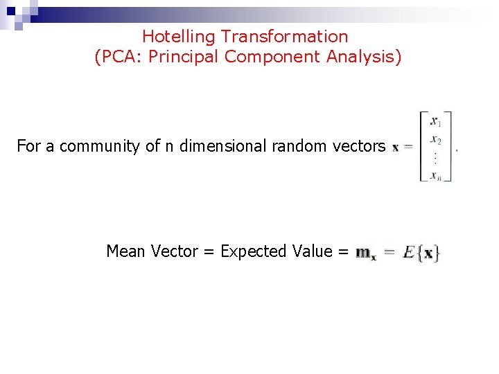
Hotelling Transformation (PCA: Principal Component Analysis) For a community of n dimensional random vectors Mean Vector = Expected Value =

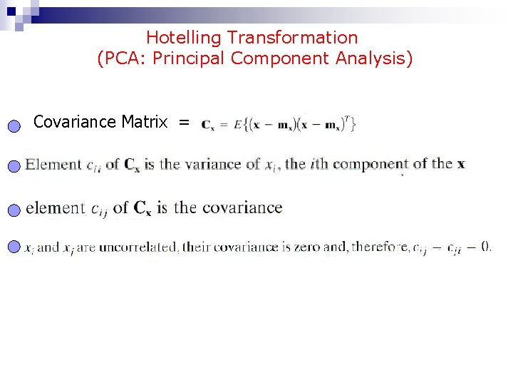
Hotelling Transformation (PCA: Principal Component Analysis) Covariance Matrix =

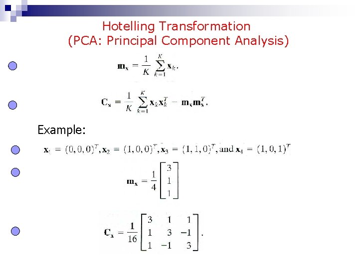
Hotelling Transformation (PCA: Principal Component Analysis) Example:

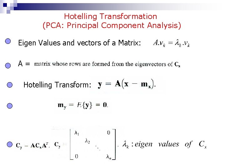
Hotelling Transformation (PCA: Principal Component Analysis) Eigen Values and vectors of a Matrix: A= Hotelling Transform:

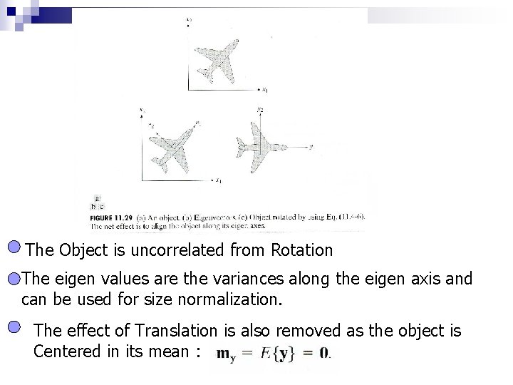
The Object is uncorrelated from Rotation The eigen values are the variances along the eigen axis and can be used for size normalization. The effect of Translation is also removed as the object is Centered in its mean :