Overview Chisquare showed us how to determine whether

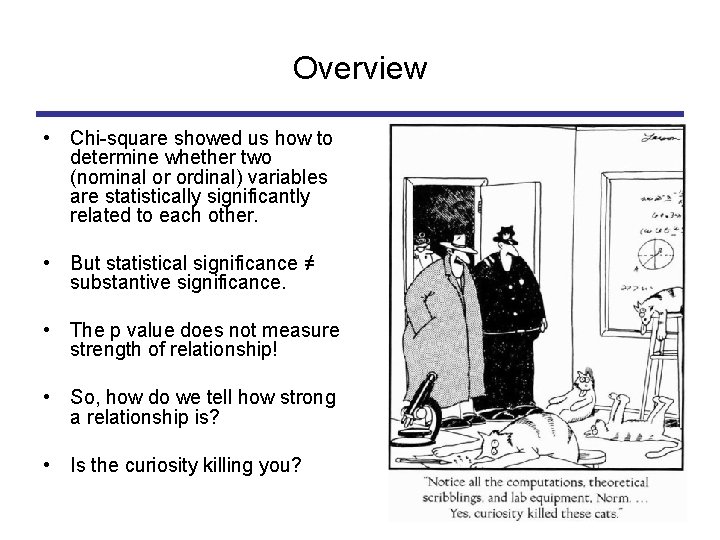
Overview • Chi-square showed us how to determine whether two (nominal or ordinal) variables are statistically significantly related to each other. • But statistical significance ≠ substantive significance. • The p value does not measure strength of relationship! • So, how do we tell how strong a relationship is? • Is the curiosity killing you?

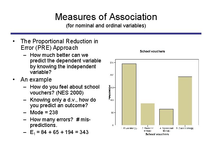
Measures of Association (for nominal and ordinal variables) • The Proportional Reduction in Error (PRE) Approach – How much better can we predict the dependent variable by knowing the independent variable? • An example – How do you feel about school vouchers? (NES 2000) – Knowing only a d. v. , how do you predict an outcome? – Mode = 238 – How many errors? # mispredictions. – E 1 = 84 + 65 + 194 = 343

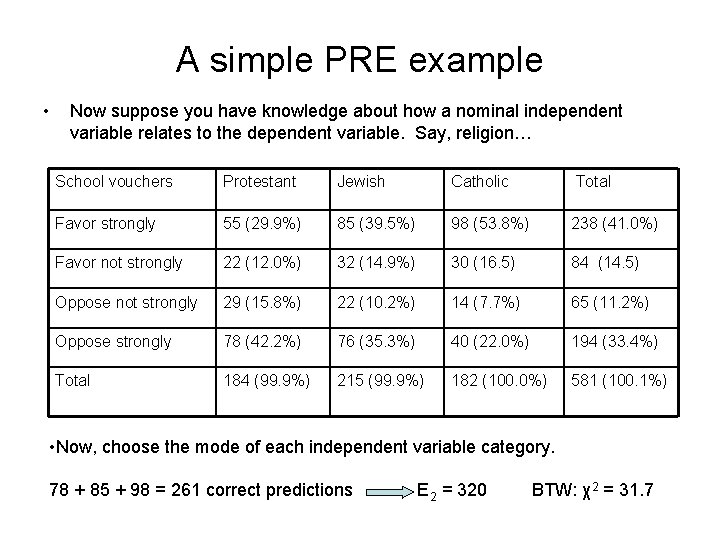
A simple PRE example • Now suppose you have knowledge about how a nominal independent variable relates to the dependent variable. Say, religion… School vouchers Protestant Jewish Catholic Total Favor strongly 55 (29. 9%) 85 (39. 5%) 98 (53. 8%) 238 (41. 0%) Favor not strongly 22 (12. 0%) 32 (14. 9%) 30 (16. 5) 84 (14. 5) Oppose not strongly 29 (15. 8%) 22 (10. 2%) 14 (7. 7%) 65 (11. 2%) Oppose strongly 78 (42. 2%) 76 (35. 3%) 40 (22. 0%) 194 (33. 4%) Total 184 (99. 9%) 215 (99. 9%) 182 (100. 0%) 581 (100. 1%) • Now, choose the mode of each independent variable category. 78 + 85 + 98 = 261 correct predictions E 2 = 320 BTW: χ2 = 31. 7

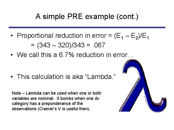
A simple PRE example (cont. ) • Proportional reduction in error = (E 1 – E 2)/E 1 = (343 – 320)/343 =. 067 • We call this a 6. 7% reduction in error… • This calculation is aka “Lambda. ” Note – Lambda can be used when one or both variables are nominal. It bombs when one dv category has a preponderance of the observations (Cramér’s V is useful then).

PRE with two ordinal variables • When both variables are ordinal, you have many options for measuring the strength of a relationship • Gamma, Kendall’s tau-b, Kendall’s tau-c, etc. • Choices, choices…

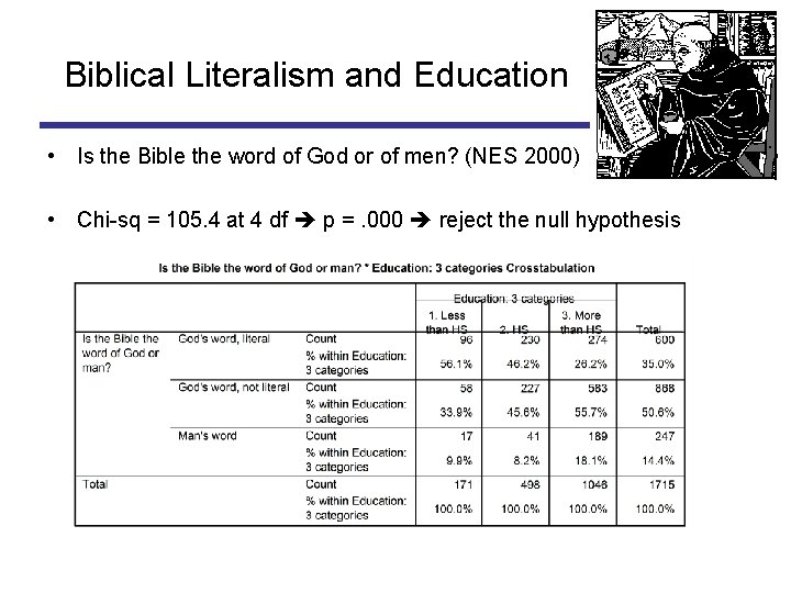
Biblical Literalism and Education • Is the Bible the word of God or of men? (NES 2000) • Chi-sq = 105. 4 at 4 df p =. 000 reject the null hypothesis

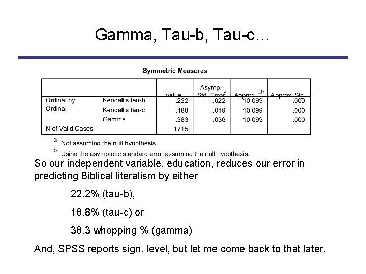
Gamma, Tau-b, Tau-c… So our independent variable, education, reduces our error in predicting Biblical literalism by either 22. 2% (tau-b), 18. 8% (tau-c) or 38. 3 whopping % (gamma) And, SPSS reports sign. level, but let me come back to that later.

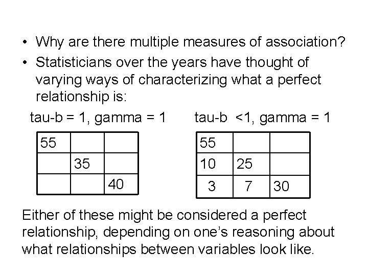
• Why are there multiple measures of association? • Statisticians over the years have thought of varying ways of characterizing what a perfect relationship is: tau-b = 1, gamma = 1 tau-b <1, gamma = 1 55 35 40 55 10 25 3 7 30 Either of these might be considered a perfect relationship, depending on one’s reasoning about what relationships between variables look like.

I’m so confused!!

Rule of Thumb • Gamma tends to overestimate strength but gives an idea of upper boundary. • If table is square use tau-b; if rectangular, use tau-c. • Pollock (and we agree): τ <. 1 is weak; . 1<τ<. 2 is moderate; . 2<τ<. 3 moderately strong; . 3< τ<1 strong.

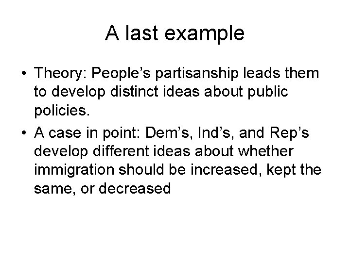
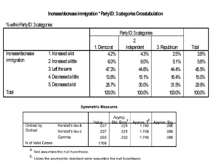
A last example • Theory: People’s partisanship leads them to develop distinct ideas about public policies. • A case in point: Dem’s, Ind’s, and Rep’s develop different ideas about whether immigration should be increased, kept the same, or decreased

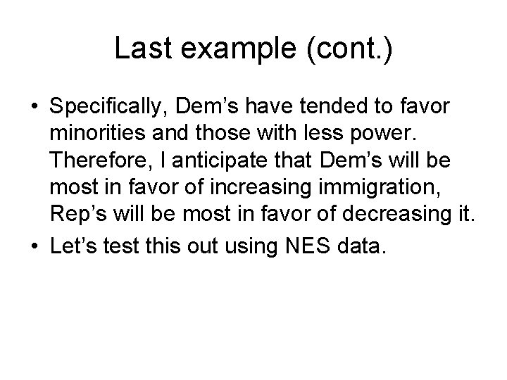
Last example (cont. ) • Specifically, Dem’s have tended to favor minorities and those with less power. Therefore, I anticipate that Dem’s will be most in favor of increasing immigration, Rep’s will be most in favor of decreasing it. • Let’s test this out using NES data.

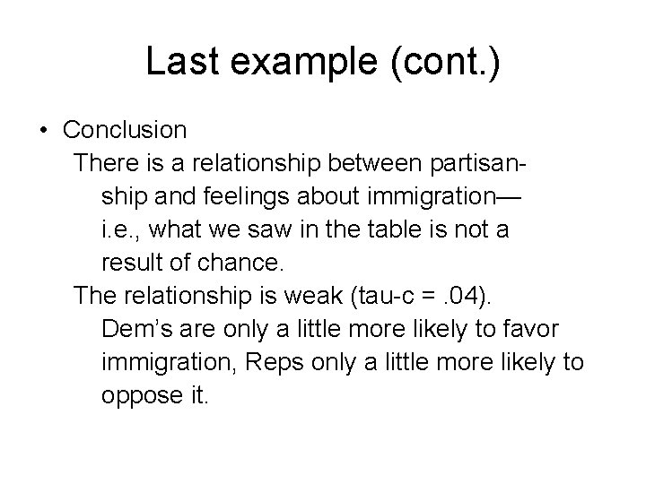
Last example (cont. ) • Conclusion There is a relationship between partisanship and feelings about immigration— i. e. , what we saw in the table is not a result of chance. The relationship is weak (tau-c =. 04). Dem’s are only a little more likely to favor immigration, Reps only a little more likely to oppose it.