Overfitting and Its Avoidance Chapter 5 Overfitting When

Overfitting and Its Avoidance 過度配適以及如何避免 Chapter 5

Overfitting過度配適 • When we build a predictive model (tree or mathematical function), we try to fit our model to data, but we don’t want ‘overfit’. 當 我們建好一個預測模型(樹或是數學函式)， 我們會試著將模型與資料搭配，但我們不 能‘過度配適’。

參數化建模 (parameter modeling)

決策樹 (decision tree)

Overfitting過度配適 • When our learner outputs a classification that is 100% accurate on the training data but 50% accurate on test data, when in fact it could have output one that is 70% accurate on both, it has overfit. 當我們的分類模型在訓練資料 集有90%的準確度，而在驗證資料集卻只有 60%，實際上它可以使兩者的準確度都達到 70%，代表這個模型已經過度配適。

Overfitting過度配適 • We want models to apply not just to the exact training set but to the general population from which the training data came. 我們希望模型不 只能運用在特定的訓練資料集，也能應用到一 般資料，而訓練資料只是其中一部分 • All data mining procedures have the tendency to overfit to some extent—some more than others. 所有的資料探勘方法在某種程度上都有過度配 適的傾向，有些比其他的更嚴重

Overfitting過度配適 • The answer is not to use a data mining procedure that doesn’t overfit because all of them do. 所以我們不是使用沒有過度配適的 資料探勘方法，因為所有都有過度配適的 問題

Overfitting過度配適 • Nor is the answer to simply use models that produce less overfitting, because there is a fundamental trade-off between model complexity and the possibility of overfitting. 也不 是使用較少過度配適的模型，其實在模型的複 雜度與過度配適的可能性之間存在著基本的利 弊權衡 • The best strategy is to recognize overfitting and to manage complexity in a principled way. 最好 的方法是去辨識過度配適，並且用有原則的方 式去管理模型複雜度。

Holdout data 預留數據 • Because evaluation on training data provides no assessment of how well the model generalizes to unseen cases, what we need to do is to “hold out” some data for which we know the value of the target variable, but which will not be used to build the model. 因為用訓練資料做評估並不能了解模型預測結果的 好壞，我們需要做的是”保有”一些我們知道目標變 數的資料，並且這些資料不會拿去建模。 • Creating holdout data is like creating a “lab test” of generalization performance. 保有這些資料就像是創 造一個”實驗室測試”，為了去了解模型普遍的表現

Holdout data 預留數據 • We will simulate the use scenario on these holdout data: we will hide from the model (and possibly the modelers) the actual values for the target on the holdout data. 我們將模 擬這些預留數據的使用場景：我們將隱藏 模型(可能還有建模者)預留數據上目標的實 際值 • The model will predict the values. 模型將會預 測這個目標值

Holdout data 預留數據 • Then we estimate the generalization performance by comparing the predicted values with the hidden true values 接著我們 會藉由比較預測值與實際值去估算模型普 遍的表現 • Thus, when the holdout data are used in this manner, they often are called the “test set. ” 因此，當預留數據被這樣使用，通常被稱 為測試資料集。

Overfitting Examined檢視過度配適 • This figure shows the difference between a modeling procedure’s accuracy on the training data and the accuracy on holdout data as model complexity changes. 這張圖片呈現了訓練 資料集與預留數據集 的準確度隨著模型複 雜度改變的變化情形 Figure 1. A typical fitting graph.

Overfitting in Tree Induction 樹狀模型的過度配適 • Recall how we built tree-structured models for classification. 回想一下我們如何建立一個分類 樹模型。 • If we continue to split the data, eventually the subsets will be pure—all instances in any chosen subset will have the same value for the target variable. These will be the leaves of our tree. 如 果我們持續切割資料，直到每個子集合最純， 每個子集都有同樣的目標值，這些是樹的葉節 點。 Figure 3. A typical fitting graph for tree induction.

Overfitting in Tree Induction 樹狀模型的過度配適 • Any training instance given to the tree for classification will make its way down, eventually landing at the appropriate leaf. 任 何一個為建立分類樹的訓練資料，會隨著 樹的分支持續往下走，最後落於適當的葉 節點 Figure 3. A typical fitting graph for tree induction.

Overfitting in Tree Induction 樹狀模型的過度配適 • It will be perfectly accurate, predicting correctly the class for every training instance. 這將會產生完美的準確度，每個訓練資料 都得到正確的預測目標值 Figure 3. A typical fitting graph for tree induction.

Overfitting in Tree Induction 樹狀模型的過度配適 • A procedure that grows trees until the leaves are pure tends to overfit. 讓樹生長直到葉節點都變純 會容易造成過度配適 • This figure shows a typical fitting graph for tree induction. 這張圖就是一個典型 樹的配適圖 Figure 3. A typical fitting graph for tree induction.

Overfitting in Tree Induction 樹狀模型的過度配適 • At some point (sweet spot) the tree starts to overfit: it acquires details of the training set that are not characteristic of the population in general, as represented by the holdout set. 在某個點(甜蜜點)樹開始 過度配適: 它取得了訓練集 的細節，但卻不是母體 的特徵，如預留數據所 顯示的 Figure 3. A typical fitting graph for tree induction.

Overfitting in Mathematical Functions 數學函式的過度配適 • As we add more Xi, the function becomes more and more complicated. 當我們加入更多的Xi，這個函式就變得更加 複雜 • Each Xi has a corresponding Wi, which is a learned parameter of the model. 每個Xi都有一個對應的Wi，是 模型中要學習的參數 • In two dimensions you can fit a line to any two points and in three dimensions you can fit a plane to any three points. 在二維空間，你可以用一條線去配適任何兩個點，在三 維空間，你可以用一個平面去配適任何三個點

Overfitting in Mathematical Functions 數學函式的過度配適 • This concept generalizes: as you increase the dimensionality, you can perfectly fit larger and larger sets of arbitrary points. 這個概念代表: 當 你增加維度，你可以完美的配適更大任意的點 集合。 • And even if you cannot fit the dataset perfectly, you can fit it better and better with more dimensions---that is, with more attributes. 即便 無法完美的配適一個資料集，你也是可以藉由 更多的維度而配適得更好，就是說，利用更多 的屬性。

Example: Overfitting Linear Functions 例子: 過度配適的線性函數 Data：sepal width, petal width 資料：萼片寬度，花瓣寬度 Types：Iris Setosa, Iris Versicolor 類型：山鳶尾，變色鳶尾 Two different separation lines： 兩種不同的線 a. Logistic regression a. 羅吉斯回歸 b. Support vector machine b. 支援向量機 Figure 5 -4

Example: Overfitting Linear Functions 例子: 過度配適的線性函數 Figure 5 -4 Figure 5 -5

Example: Overfitting Linear Functions 例子: 過度配適的線性函數 Figure 5 -4 Figure 5 -6

Overfitting in Mathematical Functions 數學函式的過度配適 • In Figures 5 -5 and 5 -6, Logistic regression appears to be overfitting. 在圖 5 -5以及5 -6，羅吉斯回歸似乎有過度配 適的現象。 • Arguably, the examples introduced in each are outliers that should not have a strong influence on the model---they contribute little to the “mass” of the species examples. 照 理說，在每個例子中引入的樣本都是異常值，不應該對 模型產生強烈影響---它們對主體樣本貢獻很小。 • Yet in the case of LR they clearly do. The SVM tends to be less sensitive to individual examples. 然而，對LR而言，顯 然那些異常值的確產生了影響，但SVM就不那麼敏感了。

Example: Overfitting Non-Linear Functions 例子: 過度配適的非線性函數 Added additional feature Sepal width 2, which gives a boundary that’s a parabola. Figure 6 Figure 7

Example: Why is Overfitting Bad? 例子: 為什麼過度配適不好? • The short answer is that as a model gets more complex it is allowed to pick up harmful spurious correlations. 簡單來說，隨著模型 變得越複雜，可能會帶進有害的假相關性。 • These correlations are idiosyncrasies of the specific training set used and do not represent characteristics of the population in general. 這些相關性是所用訓練集的特質，並不代 表一般母體的特徵。

Example: Why is Overfitting Bad? 例子: 為什麼過度配適不好? • The harm occurs when these spurious correlations produce incorrect generalizations in the model. 當這些假的相關在模型中產生 不正確的普遍化規則時，傷害就會發生。 • This is what causes performance to decline when overfitting occurs. 這是過度配適發生 時導致模型表現不好的原因。

Example: Why is Overfitting Bad? 例子: 為什麼過度配適不好? • Consider a simple two-class problem with classes c 1 and c 2 and attributes x and y. 我們 看一個簡單的兩類分類問題，類別為c 1以及 c 2，屬性值為x以及y。 • We have a population of examples, evenly balanced between the classes. 我們的樣本母 體，假設兩類平衡。

Example: Why is Overfitting Bad? 例子: 為什麼過度配適不好? • Attribute x has two values, p and q, and y has two values, r and s. 屬性x有兩種值p以及q， 屬性y有兩種值r以及s。 • In the general population, x = p occurs 75% of the time in class c 1 examples and in 25% of the c 2 examples, so x provides some prediction of the class. 在母體中，c 1的案例 有75%機會是x=p, c 2的案例有25%機會是x=p, 所以x對預測案例的類別提供某些訊息

Example: Why is Overfitting Bad? 例子: 為什麼過度配適不好? • By design, y has no predictive power at all, and indeed we see that in the data sample both of y’s values occur in both classes equally. 通過設 計，y毫無預測能力，我們看到在資料樣本 中，兩種y值都同樣出現在兩個類別中。

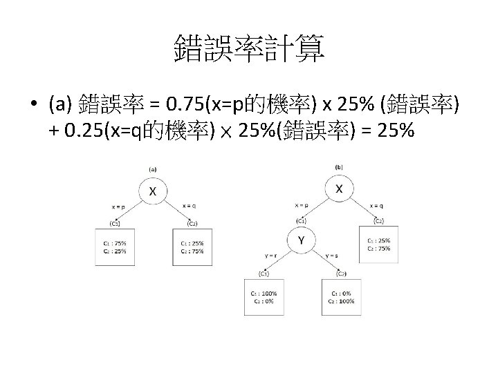
Example: Why is Overfitting Bad? 例子: 為什麼過度配適不好? • In short, the instances in this domain are difficult to separate, with only x providing some predictive power. The best we can achieve is 75% accuracy by looking at x. 簡言 之，這個case的兩種案例很難區分，只有x 提供了一些預測能力。 通過查看x，我們可 以達到的最佳準確度為 75％。

Example: Why is Overfitting Bad? 例子: 為什麼過度配適不好? • Table 5 -1 shows a very small training set of examples from this domain. What would a classification tree learner do with these? 表 5 -1呈現了這 個case的一個非常小的訓練集。 分類樹學習器將如何處理這個問題？ Table 5 -1. A small set of training examples Instance x y Class 1 p r c 1 2 p r c 1 3 p r c 1 4 q s c 1 5 p s c 2 6 q r c 2 7 q s c 2 8 q r c 2

Example: Why is Overfitting Bad? 例子: 為什麼過度配適不好? • We first obtain the tree on the left: 我們首先得到左邊的樹

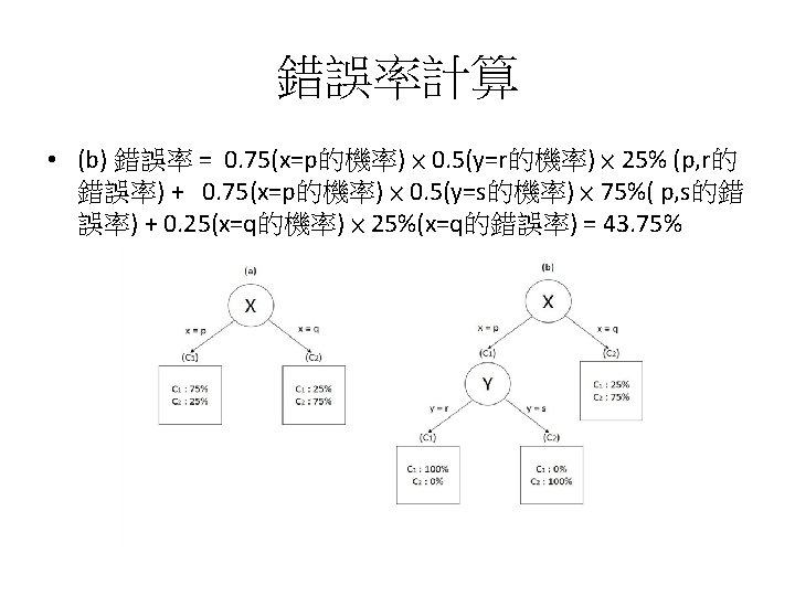
Example: Why is Overfitting Bad? 例子: 為什麼過度配適不好? • • However, observe from Table 5 -1 that in this particular dataset y’s values of r and s are not evenly split between the classes, so y does seem to provide some predictiveness. 然而，從表 5 -1可以看出，在這個特定資料集中，y的值r以及s 不是在兩類之間平均分配的，所以y似乎提供了一些預測性。 Specifically, once we choose x=p, we see that y=r predicts c 1 perfectly (instances 13). 具體來說，一旦我們選擇x = p，我們可以看到y = r完美地預測了c 1（實例1 -3）。 Table 5 -1. A small set of training examples Instance x y Class 1 p r c 1 2 p r c 1 3 p r c 1 4 q s c 1 5 p s c 2 6 q r c 2 7 q s c 2 8 q r c 2

Example: Why is Overfitting Bad? 例子: 為什麼過度配適不好? • Hence, from this dataset, tree induction would achieve information gain by splitting on y’s values and create two new leaf nodes, shown in the right tree. 因 此，從這個數據集中，樹歸納會通過分割y的值獲得信息增益，並創建兩個新 的葉節點，如右樹所示。

Example: Why is Overfitting Bad? 例子: 為什麼過度配適不好? • Based on our training set, the right tree performs well, better than the left tree. It classifies seven of the eight training examples correctly, whereas the left tree classifies only six out of eight correct. 根據我們的訓練集，右邊的樹表現良好， 比左側的樹更好。 它正確地對八個訓練樣本中的七個進行分類，而左側樹只 對八個分類中的六個進行正確分類。

Example: Why is Overfitting Bad? 例子: 為什麼過度配適不好? • But this is due to the fact that y=r purely by chance correlates with class c 1 in this data sample; in the general population there is no such correlation. 但這是由於這樣一個事實：在這個數據樣本 中，y = r純粹偶然與c 1類相關; 在一般母體資料中沒有這種相關 性。 Table 5 -1. A small set of training examples Instance x y Class 1 p r c 1 2 p r c 1 3 p r c 1 4 q s c 1 5 p s c 2 6 q r c 2 7 q s c 2 8 q r c 2

Example: Why is Overfitting Bad? 例子: 為什麼過度配適不好? • We have been misled, and the extra branch in right tree is not simply extraneous, it is harmful. 我們被誤導了，右邊樹的 額外分支不只是額外的，它是有害的。

Summary • First, this phenomenon is not particular to classification trees. Trees are convenient for this example because it is easy to point to a portion of a tree and declare it to be spurious, but all model types are susceptible to overfitting effects. 首先，這種現象並不是特 定於分類樹。樹這個例子很方便解釋，因 為我們很容易指向樹的某一部分並指出它 是假的，但是所有的模型種類都會受到過 度配適影響。

Summary • Second, this phenomenon is not due to the training data in Table 5 -1 being atypical or biased. Every dataset is a finite sample of a larger population, and every sample will have variations even when there is no bias in the sampling. 其次，這個現像不是由於表 5 -1中 的訓練資料是非典型的或有偏見的。 每個 資料集都是一個較大母體的有限樣本，即 使取樣沒有偏差，每個樣本也會有變化。

Summary • Finally, as we have said before, there is no general analytic way to determine in advance whether a model has overfit or not. 最後，正如 我們之前所說的，沒有一種通用的分析方法可 以預先確定一個模型是否有過度配適。 • In this example we defined what the population looked like so we could declare that a given model had overfit. 在這個例子中，我們定義了 母體的樣子，所以我們可以確定特定的模型有 過度配適。

Summary • In practice, you will not have such knowledge and it will be necessary to use a holdout set to detect overfitting. 在實務上，你不會知道母 體資料的情況，因此有必要使用預留數據 集來檢查過度配適。

Overfitting 詼諧版

From Holdout Evaluation to Cross-Validation 從維持評估到交叉驗證 • At the beginning of this chapter we introduced the idea that in order to have a fair evaluation of the generalization performance of a model, we should estimate its accuracy on holdout data—data not used in building the model, but for which we do know the actual value of the target variable. 在本章開頭，我們 介紹了這樣的觀點：為了對模型的整體性能進行公 平評估，我們應該估計它在預留數據方面的準確度 – 該數據沒有用在構建模型，但我們知道目標變數 的實際值。 • Holdout testing is similar to other sorts of evaluation in a “laboratory” setting. 預留測試類似於“實驗室”環 境中其他類型的評估。

From Holdout Evaluation to Cross-Validation 從維持評估到交叉驗證 • While a holdout set will indeed give us an estimate of generalization performance, it is just a single estimate. Should we have any confidence in a single estimate of model accuracy? 雖然預留數據確實給我們一個整 體性能的估計，但它只是一個單一的估計。 我們是否應該對模型準確度的單一估計有 信心？

Cross-Validation交叉驗證 • Cross-validation is a more sophisticated holdout training and testing procedure. 交叉 驗證是一個更先進的訓練和測試方法 • Cross-validation makes better use of a limited dataset. 交叉驗證可以更好地使用有限的數 據集

Cross-Validation交叉驗證 • Unlike splitting the data into one training and one holdout set, cross-validation computes its estimates over all the data by performing multiple splits and systematically swapping out samples for testing. 跟將資料分割為一個 訓練集和一個測試集方法不同，交叉驗證 通過執行多個拆分並系統地交換樣本以進 行測試來計算其對所有資料的估計。

Cross-Validation交叉驗證 • Cross-validation begins by splitting a labeled dataset into k partitions called folds. 交叉驗 證首先將標記的資料集分成稱為fold的k個 分區。 • Typically, k will be five or ten. 通常k是五或十。

Cross-Validation交叉驗證 • The top pane of Figure 5 -9 shows a labeled dataset (the original dataset) split into five folds. 圖 5 -9的上方 方塊顯示了一個有標記的資料集（原始資料集）分 成五個折疊。 • Cross-validation then iterates training and testing k times, in a particular way. 交叉驗證然後以特定的方 式迭代訓練和測試k次。 • As depicted in the bottom pane of Figure 5 -9, in each iteration of the cross-validation, a different fold is chosen as the test data. 如圖 5 -9下方方塊所示，在交 叉驗證的每次迭代中，選擇不同的fold作為測試數據。

Cross-Validation交差驗證 • In this iteration, the other k– 1 folds are combined to form the training data. 在這個迭 代中，其他k-1個fold構成訓練資料。 • So, in each iteration we have (k– 1)/k of the data used for training and 1/k used for testing. 因此，在每次迭代中，我們將（k-1）/ k的 資料用於訓練，1 / k的資料用於測試。

From Holdout Evaluation to Cross-Validation 從維持評估到交叉驗證 Holdout Evaluation Splits the data into only one training and one holdout set. 預留評估將資料分成一個訓練集和一 個預留集。 Cross-validation computes its estimates over all the data by performing multiple splits and systematically swapping out samples for testing. ( k folds, typically k would be 5 or 10. ) 交叉驗證通過執行多個拆分並系統 地交換樣本進行測試來計算其對所 有資料的估計。 （k fold，通常k是 5 或 10）。

The Churn Dataset Revisited 再看顧客流失資料集 • Consider again the churn dataset introduced in “Example: Addressing the Churn Problem with Tree Induction” on page 73. 讓我們再次看第 73頁“範例： 用樹歸納法解決客戶流失問題”中介紹的客戶流失 資料集。 • In that section we used the entire dataset both for training and testing, and we reported an accuracy of 73%. 在這一節中，我們使用整個資料集進行訓練 和測試，並且我們的準確度是 73％。 • We ended that section by asking a question, Do you trust this number? 在最後，我們問了一個問題: 你 相信這個數字嗎？

The Churn Dataset Revisited 再看顧客流失資料集

The Churn Dataset Revisited 再看顧客流失資料集 • Figure 5 -10 shows the results of ten-fold crossvalidation. In fact, two model types are shown. 圖 5 -10顯示了10 fold交叉驗證的結 果。實際上，該圖顯示了兩種模型類型。 • The top graph shows results with logistic regression, and the bottom graph shows results with classification trees. 其中上圖顯 示羅吉斯回歸的結果，下圖顯示分類樹的 結果。

The Churn Dataset Revisited 再看顧客流失資料集 • To be precise: the dataset was first shuffled, then divided into ten partitions. 準確地說：資料集 首先被洗牌，然後被分成十個分區。 • Each partition in turn served as a single holdout set while the other nine were collectively used for training. 每個分區輪流作為一個單一的預留 資料集，而其他九個共同用於訓練。 • The horizontal line in each graph is the average of accuracies of the ten models of that type. 圖中的 水平線是該類型的十個模型的平均準確度。

Observations觀察 • • “Example: Addressing the Churn Problem with Tree Induction” in Chapter 3. Average accuracy of the folds with classification trees is 68. 6%— significantly lower than our previous measurement of 73%. 分類樹fold的平均準確度為 68. 6％， 明顯低於我們先前測量的73％。 This means there was some overfitting occurring with the classification trees, and this new (lower) number is a more realistic measure of what we can expect. 這意味分類樹會出現一些過度配 適，而這個新的（較低的）數值 是我們可以預期的更現實的度量。

Observations觀察 • • “Example: Addressing the Churn Problem with Tree Induction” in Chapter 3. For accuracy with classification trees, there is variation in the performances in the different folds (the standard deviation of the fold accuracies is 1. 1), and thus it is a good idea to average them to get a notion of the performance as well as the variation we can expect from inducing classification trees on this dataset. 對於分類樹的準確度，不同fold的 表現會有所不同（準確度的標準 偏差為 1. 1），因此取平均以獲得 績效表現及變化是一個好做法， 也是我們從這個資料集建立分類 樹可以期望看到的結果

Observations觀察 • • “Example: Addressing the Churn Problem with Tree Induction” in Chapter 3. The logistic regression models show slightly lower average accuracy (64. 1%) and with higher variation (standard deviation of 1. 3 ) 邏輯回歸模型的平均準確度略低 （64. 1％），變異更大（標準差 為 1. 3）

Observations觀察 • • “Example: Addressing the Churn Problem with Tree Induction” in Chapter 3. Neither model type did very well on Fold Three and both performed well on Fold Ten. 在第三fold上這兩種模型都沒有 很好的表現，並且在第十fold上 表現都很好。 Classification trees may be preferable to logistic regression because of their greater stability and performance. 由於分類樹具有較高的穩定性和性 能，因此可能比羅吉斯回歸更適合。

Learning Curves學習曲線 • • All else being equal, the generalization performance of data-driven modeling generally improves as more training data become available, up to a point. 在其他條件相同的情況下，資料導向建模的整體表現通常會隨著有更多可用訓練資 料而提昇，直至達到某一點。 (for the telecommunications churn problem)

Learning Curves學習曲線 • More flexibility in a model comes more overfitting. 模 型越彈性越容易導致過度配適。 • Logistic regression has less flexibility, which allows it to overfit less with small data, but keeps it from modeling the full complexity of the data. 羅吉斯回歸具有較小 的彈性，這使得它配適較小的資料時，overfit較小。 但對大資料，較不能將完整資料規則納入其模型內。

Learning Curves學習曲線 • Tree induction is much more flexible, leading it to overfit more with small data, but to model more complex regularities with larger training sets. • 樹歸納較為彈性，這使得它配適較小的資料時， overfit較大。但對大資料，較能夠將完整資料規則納 入其模型內。

Learning Curves學習曲線 • The learning curve has additional analytical uses. For example, we’ve made the point that data can be an asset. The learning curve may show that generalization performance has leveled off so investing in more training data is probably not worthwhile; instead, one should accept the current performance or look for another way to improve the model, such as by devising better features. • 學習曲線有其他分析用途。 例如，我們已經說過資 料是一項資產。當學習曲線顯示整體性能已趨於穩 定，投入更多訓練數據可能就不值得了; 我們要嘛接 受當前的表現，不然就需要另找改進模型的方法， 例如通過設計更好的特徵

Avoiding Overfitting with Tree Induction 使用樹狀結構時避免過度配適 • • Tree induction has much flexibility and therefore will tend to overfit a good deal without some mechanism to avoid it. 樹歸納具有很大的彈性，如果我們沒有一些機制來避免， 它會有相當程度的過度配適

Avoiding Overfitting with Tree Induction 使用樹狀結構時避免過度配適 • Tree induction commonly uses two techniques to avoid overfitting. These strategies are : (i) to stop growing the tree before it gets too complex, and (ii) to grow the tree until it is too large, then “prune” it back, reducing its size (and thereby its complexity). 樹歸納通常使用兩種技術來避免過度配適： （i）在樹變得太複雜之前停止讓樹增長 （ii）讓樹長直到它太大，然後“修剪”它，減小它的尺寸 （從而減小它的複雜度）。

To stop growing the tree before it gets too complex 在樹太複雜之前停止樹增長 • The simplest method to limit tree size is to specify a minimum number of instances that must be present in a leaf. 最簡單方法是去限制樹的大小，例如 指定葉中必須有的最小案例數。 • A key question becomes what threshold we should use. 但一個關鍵問題就是我 們該用甚麼門檻值?

To stop growing the tree before it gets too complex 在樹太複雜之前停止增長樹 • • • How few instances are we willing to tolerate at a leaf? Five instances? Thirty? One hundred? There is no fixed number, although practitioners tend to have their own preferences based on experience. 我們願意在一片葉子上容忍多麼少的案例？ 五個案 例？ 三十個？ 一百個？ 沒有甚麼固定好的數字， 但是實務從業人員傾向於根據經驗有自己的偏好。 However, researchers have developed techniques to decide the stopping point statistically. 但是，研究人 員已經開發出用統計方法決定停止點的技術。

To stop growing the tree before it gets too complex 在樹太複雜之前停止增長樹 • • For stopping tree growth, an alternative to setting a fixed size for the leaves is to conduct a hypothesis test at every leaf to determine whether the observed difference in (say) information gain could not have been due to chance, e. g. p-value <= 5%. 為了阻止樹生 長，一個替代方法是在每片樹葉進行假設檢定，目 的是確定所觀察到的信息增益差異是否不是偶然的， 例如， 檢測p值<= 5％。 If the hypothesis test concludes that it was likely not due to chance, then the split is accepted and the tree growing continues. 如果假設檢定得出結論認為這很 可能不是偶然的，那麼就進行分支，讓樹繼續生長。

To grow the tree until it is too large, then “prune” it back 增長樹直到它太大，然後“修剪”回來 • • • Pruning means to cut off leaves and branches, replacing them with leaves. 修剪意味著切掉樹葉和樹 枝，用葉子代替它們 One general idea is to estimate whether replacing a set of leaves or a branch with a leaf would reduce accuracy. If not, then go ahead and prune. 一般的做法是估計用 樹葉替換一組樹葉或樹枝是否會降低準確性。 如果 不會，那麼就進行修剪。 The process can be iterated on progressive subtrees until any removal or replacement would reduce accuracy. 這過程可以漸進在子樹上進行，直到任何 移除或替換都會降低準確度為止

A General Method for Avoiding Overfitting 一個避免過度配適的方法 Nested holdout testing: Split the original set into training and test sets. Saving the test set for a final assessment. We can take the training set and split it again into a training subset and a validation set. Use the training subset and validation set to find the best model, e. g. , tree with a complexity of 122 nodes (the “sweet spot”). 嵌套預留測試：將原始資料分為訓練和測試集。 保留測試集以進行最終評估。 我們可以將訓練集合再 分成一個訓練子集和一個驗證集。 使用訓練子集和驗證集合來找到最佳模型，例如復雜度為 122個節點 的樹（“甜蜜點”）。 • • The final holdout set is used to estimate the actual generalization performance. 最後預留資料集用於估計實際的整體性能。 One more twist: we could use the training subset & validation split to pick the best complexity without tainting the test set, and build a model of this best complexity on the entire training set (training subset plus validation). 還有一個點：我們可以使用訓練子集和驗證拆分 來找到最佳複雜度而不影響測試集，然後用整個 訓練集（訓練子集和驗證）去構建這種最佳複雜 度的模型。 This approach is used in many sorts of modeling algorithms to control complexity. The general method is to choose the value for some complexity parameter by using some sort of nested holdout procedure. 這種方法被用於許多種建模算法來控制複雜性。 一般的方法是通過使用某種嵌套預留程序來選擇一 些複雜度參數的值。 Training set Training subset Validation set Test set ( hold out ) Final holdout set

Overfitting in Tree Induction 樹狀模型的過度配適 • At some point (sweet spot) the tree starts to overfit: it acquires details of the training set that are not characteristic of the population in general, as represented by the holdout set. 在某個點(甜蜜點)樹開始 過度配適: 它取得了訓練集 的細節，但卻不是母體 的特徵，如預留數據所 顯示的 Figure 3. A typical fitting graph for tree induction.

Nested cross-validation 嵌套交叉驗證 • Nested cross-validation is more complicated, but it works as you might suspect. 嵌套交叉驗 證較為複雜，但它的運作，可能如你想的。 • Say we would like to do cross-validation to assess the generalization accuracy of a new modeling technique, which has an adjustable complexity parameter C, but we do not know how to set it. 假設我們希望進行交叉驗證來 評估新建模技術的普遍化精度，該建模技術 具有可調整的複雜度參數C，但我們不知道 如何設置它。

Nested cross-validation 嵌套交叉驗證 • So, we run cross-validation as described above. • 所以，我們如上所述進行交叉驗證。 • However, before building the model for each fold, we take the training set (refer to Figure 59) and first run an experiment: we run another entire cross validation on just that training set to find the value of C estimated to give the best accuracy. 然而，在為每一個fold構建模型之 前，我們用訓練集（參見圖 5 -9）首先做一 個實驗：我們對該訓練集進行另一個完整的 交叉驗證，找到能給出最準確的結果的C值。

Nested cross-validation 嵌套交叉驗證 • The result of that experiment is used only to set the value of C to build the actual model for that fold of the cross-validation. Then we build another model using the entire training fold, using that value for C, and test on the corresponding test fold. 該實驗的結果僅用於 設定C的值以構建交叉驗證的該fold的實際模 型。 然後我們使用整個訓練fold去構建另一 個模型，將該值用於C，並在相應的測試fold 上進行測試。

From Holdout Evaluation to Cross-Validation 從預留評估到交叉驗證 Holdout Evaluation Splits the data into only one training and one holdout set. 預留評估將資料分成只有一個訓練和 一個維持組。 Cross-validation computes its estimates over all the data by performing multiple splits and systematically swapping out samples for testing. ( k folds, typically k would be 5 or 10. ) 交叉驗證通過執行多個拆分並系統 地交換樣本進行測試來計算其對所 有資料的估計。 （k fold，通常k是 5 或 10）。

Nested Cross-Validation 嵌套交叉驗證 Training set Test set Original data

Nested cross-validation 嵌套交叉驗證 • The only difference from regular crossvalidation is that for each fold we first run this experiment to find C, using another, smaller, cross-validation. • 與一般交叉驗證唯一區別在於，對於 每一次迭代，我們首先運行此實驗以 找到C，並使用另一個較小的交叉驗證。

Nested cross-validation 嵌套交叉驗證 • • If you understood all that, you would realize that if we used 5 -fold cross-validation in both cases, we actually have built 30 total models in the process (yes, thirty). 如果你知道交叉驗證的程序，那麼你會知道，如果 我們在這兩種情況下使用了5倍交叉驗證，我們實 際上已經在此過程中建立了30個總模型（對，是 30 ）。 This sort of experimental complexity-controlled modeling only gained broad practical application over the last decade or so, because of the obvious computational burden involved. 由於明顯的較多的計算負擔，這種實驗式的複雜度 控制模型在過去十年左右才獲得廣泛的實際應用。

Nested cross-validation 嵌套交叉驗證 • • This idea of using the data to choose the complexity experimentally, as well as to build the resulting model, applies across different induction algorithms and different sorts of complexity. 這種使用數據藉實驗去 選擇複雜度以及構建最終模型的思路適用於不同的 歸納算法和不同類型的複雜性。 For example, we mentioned that complexity increases with the size of the feature set, so it is usually desirable to cull (選出) the feature set. 例如，我們提到複雜 度隨著特徵集的大小而增加，因此通常需要剔除（ 選出）特徵集。

Nested cross-validation 嵌套交叉驗證 • A common method for doing this is to run with many different feature sets, using this sort of nested holdout procedure to pick the best. • 常見方法是測試多個不同的特徵集， 使用這種嵌套維持程序來選擇最佳特 徵。

Sequential forward selection 循序向前選擇 • • For example, sequential forward selection (SFS) of features uses a nested holdout procedure to first pick the best individual feature, by looking at all models built using just one feature. 例如，順序前向選擇（ SFS）是使用嵌套維持過程首先選擇最佳單個特徵， 方法是查看僅使用一個特徵構建的所有模型。 After choosing a first feature, SFS tests all models that add a second feature to this first chosen feature. The best pair is then selected. 選擇第一個特徵後，SFS 會測試所有將第二個功能添加到第一個選定特徵的 模型。 然後選擇最好的一對。

Sequential forward selection 循序向前選擇 • Next the same procedure is done for three, then four, and so on. 接下來，同 樣的程序完成三個，然後四個，依此 類推。 • When adding a feature does not improve classification accuracy on the validation data, the SFS process stops. 當添加特徵 不會提高驗證資料的分類準確性時， SFS進程停止。

Sequential backward selection 循序向後選擇 • There is a similar procedure called sequential backward elimination of features. 一個類似的 過程稱為循序向後消除特徵。 • As you might guess, it works by starting with all features and discarding features one at a time. 正如您可能想到的那樣，它通過從所有特徵 開始並逐個丟棄特徵。 • It continues to discard features as long as there is no performance loss. 只要表現沒有變差， 它就會繼續丟棄特徵。

Nested cross-validation 嵌套交叉驗證 • This is a common approach. In modern environments with plentiful data and computational power, the data scientist routinely sets modeling parameters by experimenting using some tactical, nested holdout testing (often nested cross-validation). • 這是一種常見的方法。 在具有豐富數據和計 算能力的現代環境中，資料科學家通過使用 嵌套式預留測試（通常為嵌套交叉驗證）進 行實驗來選定建模參數。