Outline Scapegoat Trees Olog n amortized time 2

Outline • Scapegoat Trees ( O(log n) amortized time) • 2 -4 Trees ( O(log n) worst case time) • Red Black Trees ( O(log n) worst case time)

Review Skiplists and Treaps • So far, we have seen treaps and skiplists • Randomized structures • Insert/delete/search time in O(log n) expected • Expectation depends on random choices made by the data structure • Coin tosses made by a skiplist • Random priorities assigned by a treap

Scapegoat trees • Deterministic data structure • Lazy data structure • Only • Search does work when search paths get too long in O(log n) worst-case time • Insert/delete • Starting in O(log n) amortized time with an empty scapegoat tree, a sequence of m insertions and deletions takes O(mlog n) time

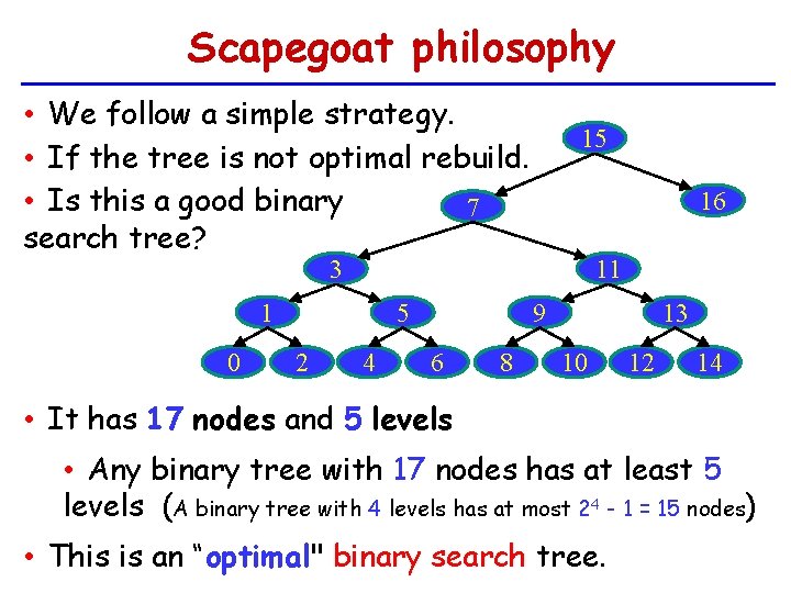
Scapegoat philosophy • We follow a simple strategy. • If the tree is not optimal rebuild. • Is this a good binary 7 search tree? 15 16 3 1 0 5 2 4 11 9 6 8 13 10 12 14 • It has 17 nodes and 5 levels • Any binary tree with 17 nodes has at least 5 levels (A binary tree with 4 levels has at most 24 - 1 = 15 nodes) • This is an “optimal" binary search tree.

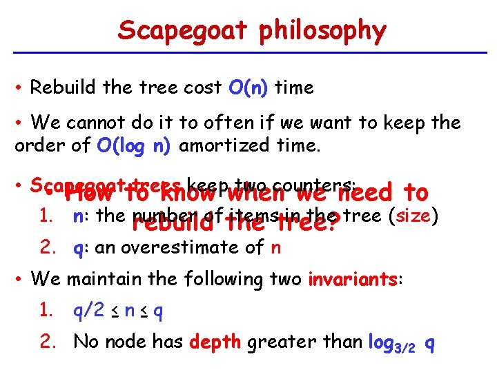
Scapegoat philosophy • Rebuild the tree cost O(n) time • We cannot do it to often if we want to keep the order of O(log n) amortized time. • Scapegoat trees keepwhen two counters: • How to know we need 1. to n: the number itemstree? in the tree (size) rebuildof the 2. q: an overestimate of n • We maintain the following two invariants: 1. q/2 ≤ n ≤ q 2. No node has depth greater than log 3/2 q

Search and Delete • How can we perform a search in a Scapegoat tree? • How can we delete a value x from a Scapegoat tree? 1. run the standard deletion algorithm for binary search trees. 2. decrement n 3. if n < q/2 then • rebuild the entire tree and set q=n • How can we insert a value x into a Scapegoat tree?

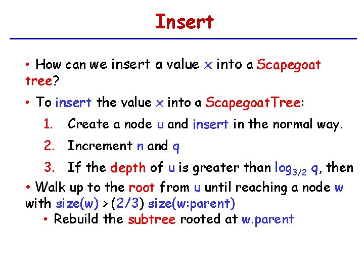
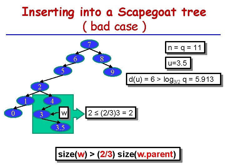
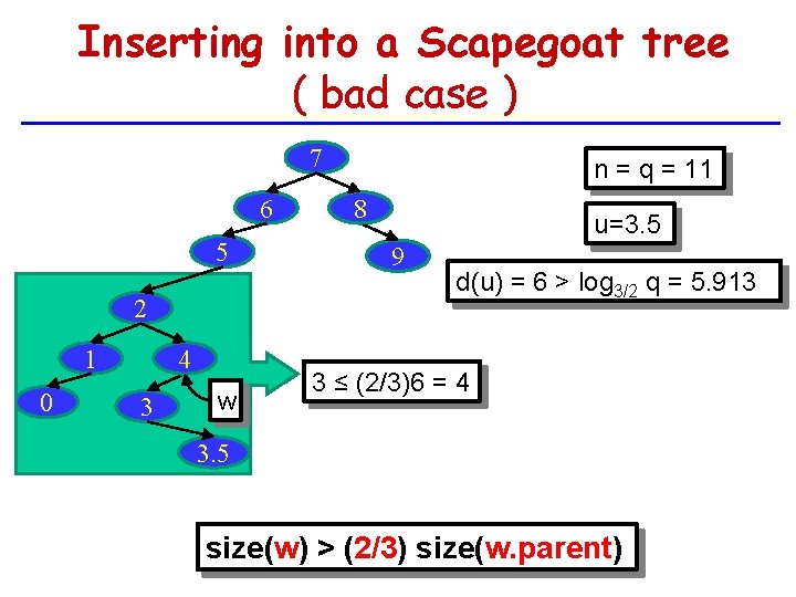
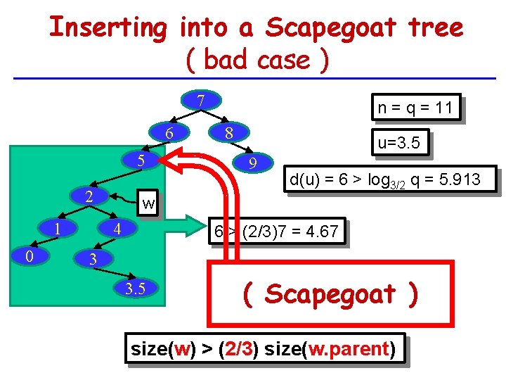
Insert • How can we insert a value x into a Scapegoat tree? • To insert the value x into a Scapegoat. Tree: 1. Create a node u and insert in the normal way. 2. Increment n and q 3. If the depth of u is greater than log 3/2 q, then • Walk up to the root from u until reaching a node w with size(w) > (2/3) size(w: parent) • Rebuild the subtree rooted at w. parent

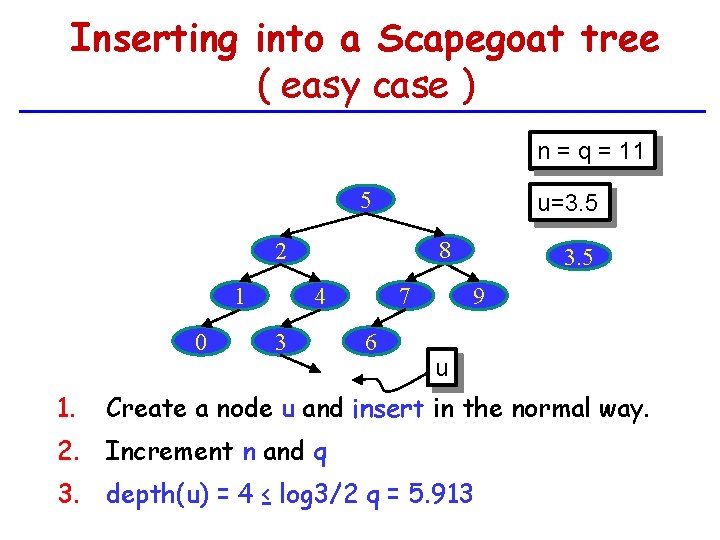
Inserting into a Scapegoat tree ( easy case ) n = q = 11 10 5 u=3. 5 8 2 1 0 1. 7 4 3 6 3. 5 9 u Create a node u and insert in the normal way. 2. Increment n and q 3. depth(u) = 4 ≤ log 3/2 q = 5. 913

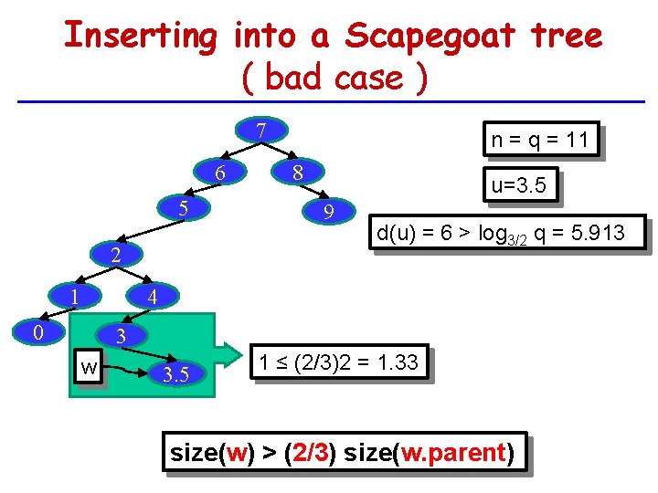
Inserting into a Scapegoat tree ( bad case ) 7 6 5 2 1 n = q = 11 8 u=3. 5 9 d(u) = 6 > log 3/2 q = 5. 913 4 0 3 w 3. 5 1 ≤ (2/3)2 = 1. 33 size(w) > (2/3) size(w. parent)

Inserting into a Scapegoat tree ( bad case ) 7 6 0 8 u=3. 5 5 9 w 2 ≤ (2/3)3 = 2 2 1 n = q = 11 d(u) = 6 > log 3/2 q = 5. 913 4 3 3. 5 size(w) > (2/3) size(w. parent)

Inserting into a Scapegoat tree ( bad case ) 7 6 5 2 1 0 4 3 w n = q = 11 8 u=3. 5 9 d(u) = 6 > log 3/2 q = 5. 913 3 ≤ (2/3)6 = 4 3. 5 size(w) > (2/3) size(w. parent)

Inserting into a Scapegoat tree ( bad case ) 7 6 5 2 1 0 n = q = 11 8 u=3. 5 9 d(u) = 6 > log 3/2 q = 5. 913 w 4 6 > (2/3)7 = 4. 67 3 3. 5 ( Scapegoat ) size(w) > (2/3) size(w. parent)

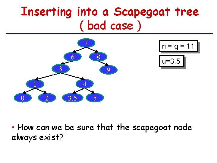
Inserting into a Scapegoat tree ( bad case ) 7 6 n = q = 11 8 3 9 4 1 0 u=3. 5 2 3. 5 5 • How can we be sure that the scapegoat node always exist?

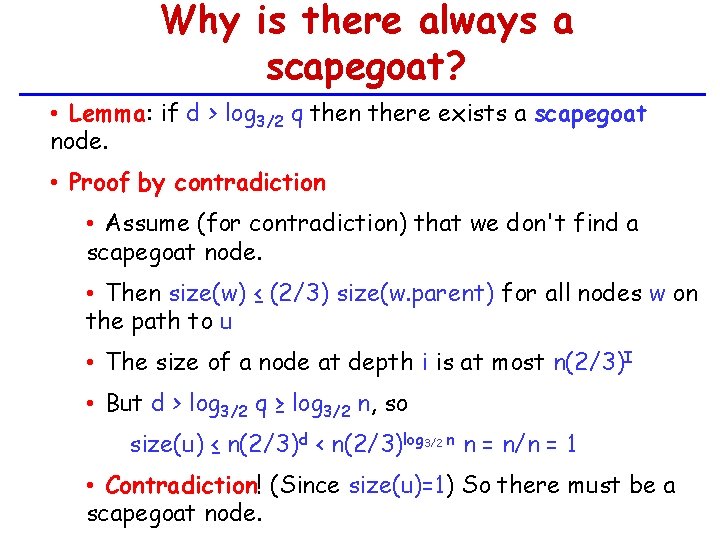
Why is there always a scapegoat? • Lemma: if d > log 3/2 q then there exists a scapegoat node. • Proof by contradiction • Assume (for contradiction) that we don't find a scapegoat node. • Then size(w) ≤ (2/3) size(w. parent) for all nodes w on the path to u • The size of a node at depth i is at most n(2/3)I • But d > log 3/2 q ≥ log 3/2 n, so size(u) ≤ n(2/3)d < n(2/3)log 3/2 n n = n/n = 1 • Contradiction! (Since size(u)=1) So there must be a scapegoat node.

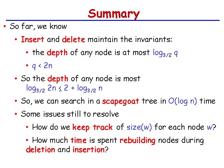
• So far, we know Summary • Insert and delete maintain the invariants: • the depth of any node is at most log 3/2 q • q < 2 n • So the depth of any node is most log 3/2 2 n ≤ 2 + log 3/2 n • So, we can search in a scapegoat tree in O(log n) time • Some issues still to resolve • How do we keep track of size(w) for each node w? • How much time is spent rebuilding nodes during deletion and insertion?

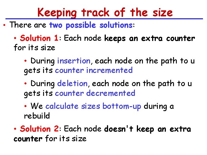
Keeping track of the size • There are two possible solutions: • Solution 1: Each node keeps an extra counter for its size • During insertion, each node on the path to u gets its counter incremented • During deletion, each node on the path to u gets its counter decremented • We calculate sizes bottom-up during a rebuild • Solution 2: Each node doesn't keep an extra counter for its size

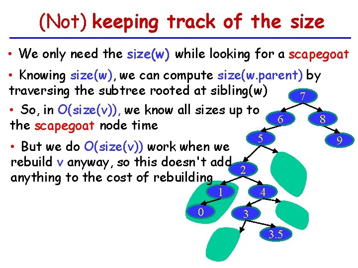
(Not) keeping track of the size • We only need the size(w) while looking for a scapegoat • Knowing size(w), we can compute size(w. parent) by traversing the subtree rooted at sibling(w) 7 • So, in O(size(v)), we know all sizes up to 6 8 the scapegoat node time • But we do O(size(v)) work when we rebuild v anyway, so this doesn't add 2 anything to the cost of rebuilding 1 0 5 9 4 3 3. 5

Analysis of deletion • When deleting, if n < q/2, then we rebuild the whole tree • This takes O(n) time • If n < q/2 then we have done at least q - n > n/2 deletions • The amortized (average) cost of rebuilding (due to deletions) is O(1) per deletion

Analysis of insertion • If no rebuild is necessary the cost of the insertion is log( n ) • After rebuilding a sub tree containing node v, both of its children have de same size*. • If the subtree rooted in v has size n we needed at least n/3 insertion the previous rebuilding process. • The rebuild cost n(log n) operations • Thus the cost of the insertion is O(log n) amortized time.

Scapegoat trees summary • Theorem: − The cost to search in a scapegoat tree is O(log n) in the worst-case. − The cost of insertion and deletion in a scapegoat tree are O(log n) amortized time per operation. • Scapegoat trees often work even better than expected • If we get lucky, then no rebuilding is required

Review: Maintaining Sorted Sets • We have seen the following data structures for implementing a Sorted. Set − Skiplists: find(x)/add(x)/remove(x) in O(log n) expected time per operation − Treaps: find(x)/add(x)/remove(x) in O(log n) expected time per operation − Scapegoat trees: find(x) in O(log n) worst-case time per operation, add(x)/remove(x) in O(log n) amortized time per operation

Review: Maintaining Sorted Sets • No data structures course would be complete without covering − 2 -4 trees: find(x)/add(x)/remove(x) in O(log n) worst-case time per operation − Red-black trees: find(x)/add(x)/remove(x) in O(log n) worst-case time per operation

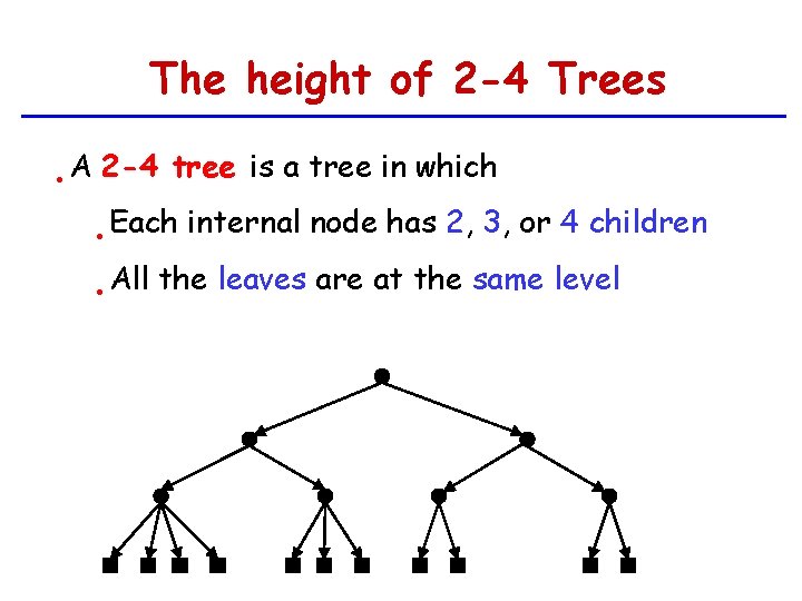
The height of 2 -4 Trees • A 2 -4 tree is a tree in which • Each • All internal node has 2, 3, or 4 children the leaves are at the same level

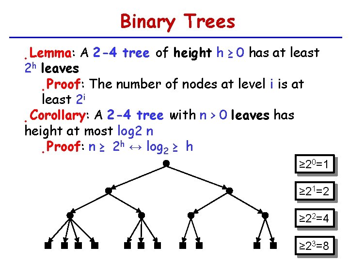
Binary Trees Lemma: A 2 -4 tree of height h ≥ 0 has at least 2 h leaves • Proof: The number of nodes at level i is at least 2 i • Corollary: A 2 -4 tree with n > 0 leaves has height at most log 2 n h ↔ log ≥ h Proof: n ≥ 2 2 • • ≥ 20=1 ≥ 21=2 ≥ 22=4 ≥ 23=8

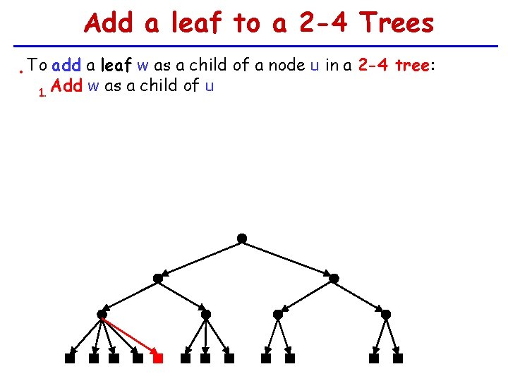
Add a leaf to a 2 -4 Trees • To add a leaf w as a child of a node u in a 2 -4 tree: Add w as a child of u 1.

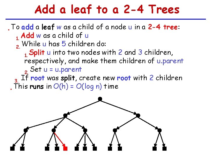
Add a leaf to a 2 -4 Trees • To add a leaf w as a child of a node u in a 2 -4 tree: Add w as a child of u 1. While u has 5 children do: 2. 1. Split u into two nodes with 2 and 3 children, respectively, and make them children of u. parent 2. Set u = u. parent If root was split, create new root with 2 children 3. • This runs in O(h) = O(log n) time

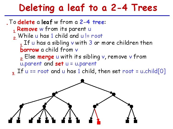
Deleting a leaf to a 2 -4 Trees • To delete a leaf w from a 2 -4 tree: Remove w from its parent u 1. While u has 1 child and u != root 2. 1. If u has a sibling v with 3 or more children then borrow a child from v 2. Else merge u with its sibling v, remove v from u. parent and set u = u. parent If u == root and u has 1 child, then set root = u. child[0] 3.

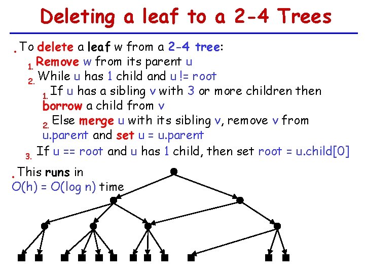
Deleting a leaf to a 2 -4 Trees • To delete a leaf w from a 2 -4 tree: Remove w from its parent u 1. While u has 1 child and u != root 2. 1. If u has a sibling v with 3 or more children then borrow a child from v 2. Else merge u with its sibling v, remove v from u. parent and set u = u. parent If u == root and u has 1 child, then set root = u. child[0] 3. This runs in O(h) = O(log n) time •

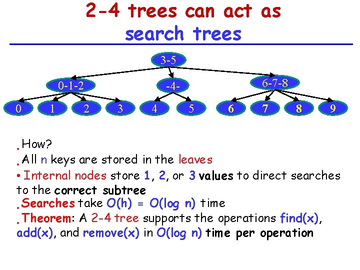
2 -4 trees can act as search trees 3 -5 0 -1 -2 0 1 2 6 -7 -8 -43 4 5 6 7 8 9 How? All n keys are stored in the leaves • • Internal nodes store 1, 2, or 3 values to direct searches to the correct subtree Searches take O(h) = O(log n) time • Theorem: A 2 -4 tree supports the operations find(x), • add(x), and remove(x) in O(log n) time per operation •

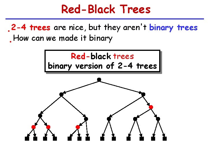
Red-Black Trees 2 -4 trees are nice, but they aren't binary trees How can we made it binary • • Red-black trees binary version of 2 -4 trees

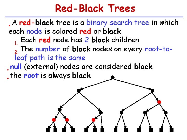
Red-Black Trees A red-black tree is a binary search tree in which each node is colored or black Each red node has 2 black children 1. The number of black nodes on every root-to 2. leaf path is the same null (external) nodes are considered black • • the root is always black •

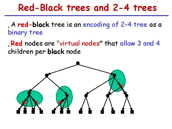
Red-Black trees and 2 -4 trees A red-black tree is an encoding of 2 -4 tree as a binary tree • Red nodes are “virtual nodes" that allow 3 and 4 children per black node •

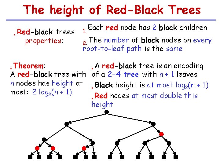
The height of Red-Black Trees Red-black trees • properties: 1. Each red node has 2 black children 2. The number of black nodes on every root-to-leaf path is the same Theorem: A red-black tree is an encoding • A red-black tree with of a 2 -4 tree with n + 1 leaves n nodes has height at • Black height is at most log 2(n + 1) most: 2 log 2(n + 1) Red nodes at most double this • height •

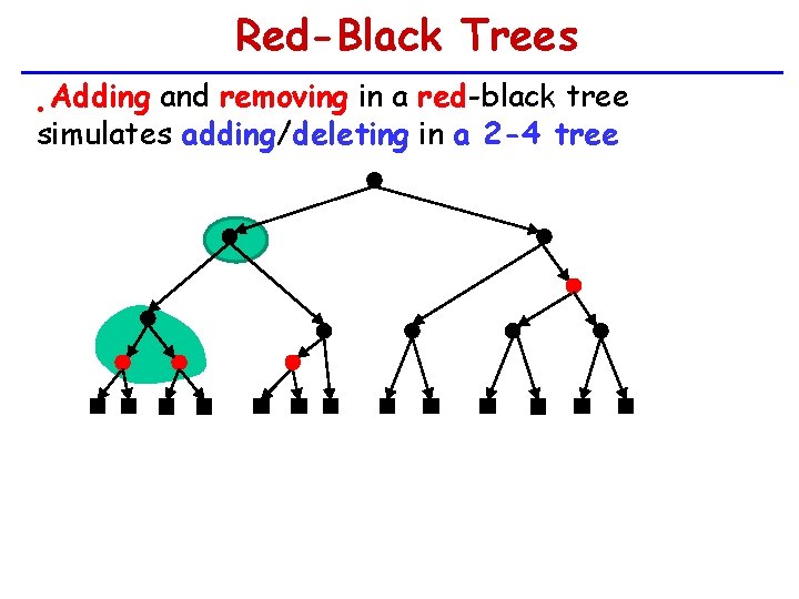
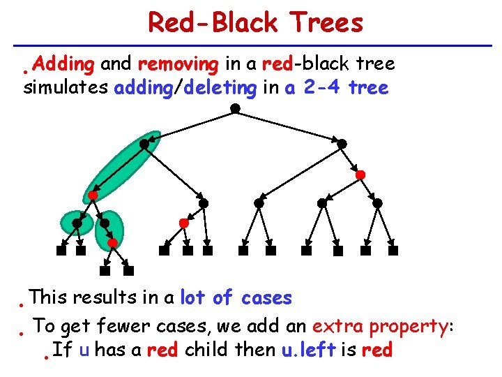
Red-Black Trees Adding and removing in a red-black tree simulates adding/deleting in a 2 -4 tree •

Red-Black Trees Adding and removing in a red-black tree simulates adding/deleting in a 2 -4 tree • This results in a lot of cases To get fewer cases, we add an extra property: • • If u has a red child then u. left is red •

Adding to a read black tree • To add a new value to a red-black tree: 1. create a new red node u and insert it as usual (as a leaf) 2. call insert. Fixup(u) to restore 1. no red-red edge 2. if u has a red child then u. left is red • Each iteration of add. Fixup(u) moves u up in tree • Finishes after O(log n) iterations in O(log n) time

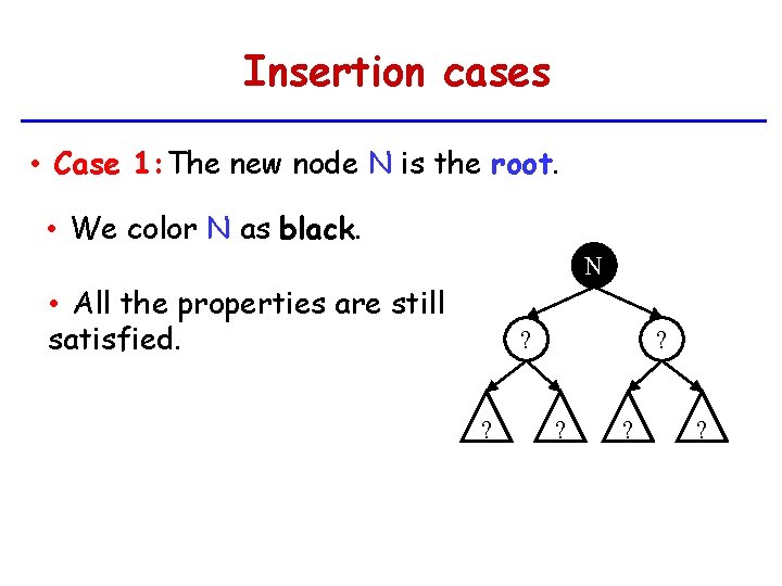
Insertion cases • Case 1: The new node N is the root. • We color N as black. N • All the properties are still satisfied. ? ? ? ?

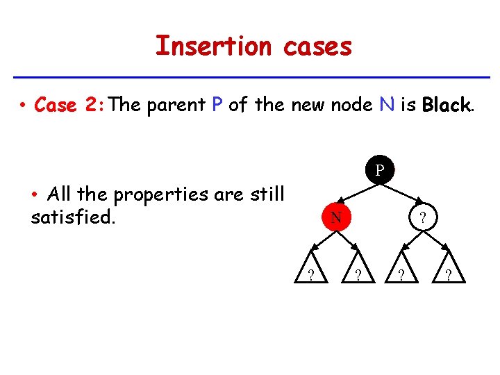
Insertion cases • Case 2: The parent P of the new node N is Black. P • All the properties are still satisfied. N ? ? ?

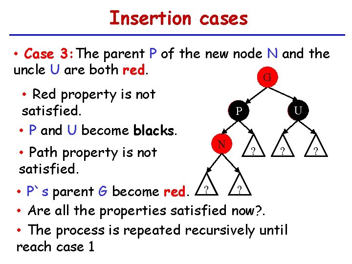
Insertion cases • Case 3: The parent P of the new node N and the uncle U are both red. G • Red property is not satisfied. • P and U become blacks. • Path property is not satisfied. G U P N ? ? ? • P`s parent G become red. ? • Are all the properties satisfied now? . • The process is repeated recursively until reach case 1 ?

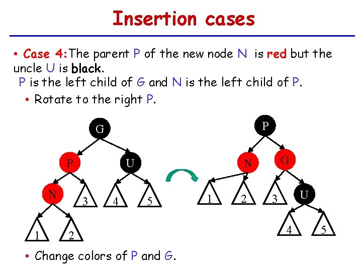
Insertion cases • Case 4: The parent P of the new node N is red but the uncle U is black. P is the left child of G and N is the left child of P. • Rotate to the right P. P G P N 1 3 4 G N U 5 2 • Change colors of P and G. 1 2 U 3 4 5

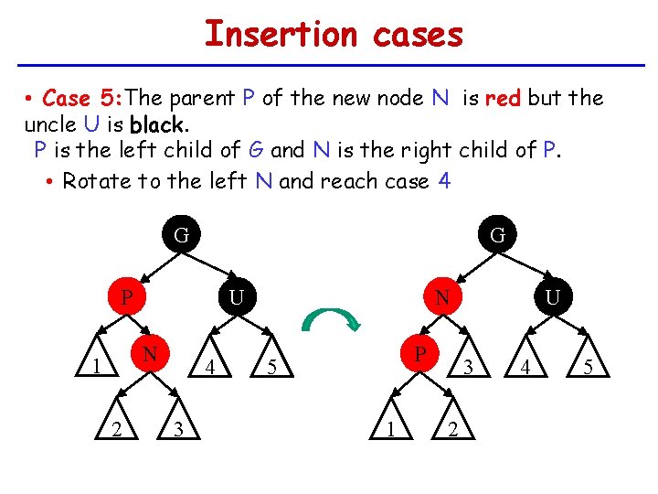
Insertion cases • Case 5: The parent P of the new node N is red but the uncle U is black. P is the left child of G and N is the right child of P. • Rotate to the left N and reach case 4 G G P N 1 2 N U 4 3 P 5 1 U 3 2 4 5

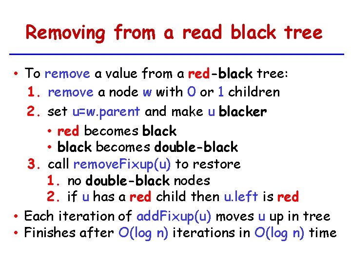
Removing from a read black tree • To remove a value from a red-black tree: 1. remove a node w with 0 or 1 children 2. set u=w. parent and make u blacker • red becomes black • black becomes double-black 3. call remove. Fixup(u) to restore 1. no double-black nodes 2. if u has a red child then u. left is red • Each iteration of add. Fixup(u) moves u up in tree • Finishes after O(log n) iterations in O(log n) time

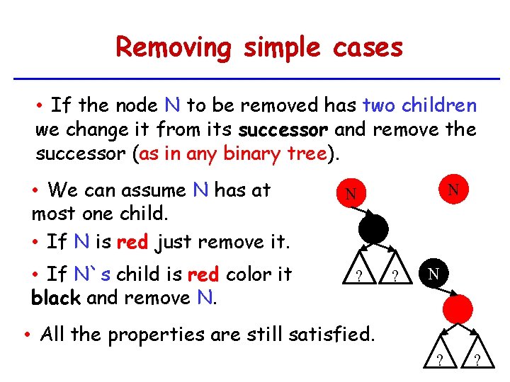
Removing simple cases • If the node N to be removed has two children we change it from its successor and remove the successor (as in any binary tree). • We can assume N has at most one child. • If N is red just remove it. • If N`s child is red color it black and remove N. N N ? ? N • All the properties are still satisfied. ? ?

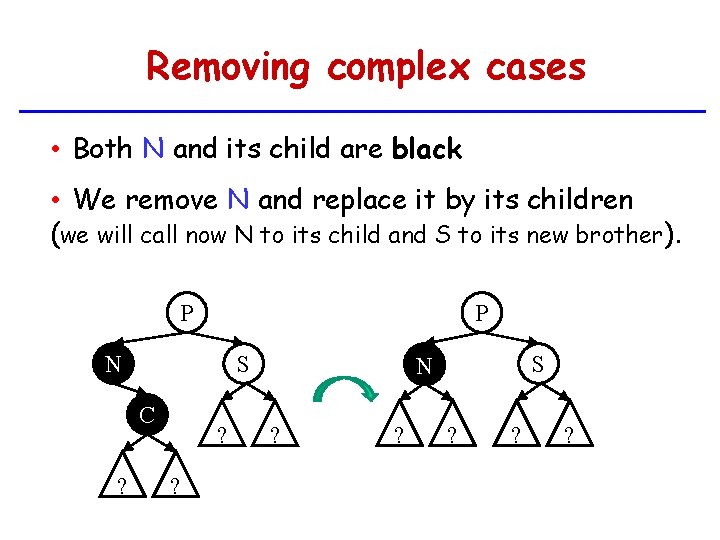
Removing complex cases • Both N and its child are black • We remove N and replace it by its children (we will call now N to its child and S to its new brother). P P N S C ? ? ? C N ? ? S ? ? ?

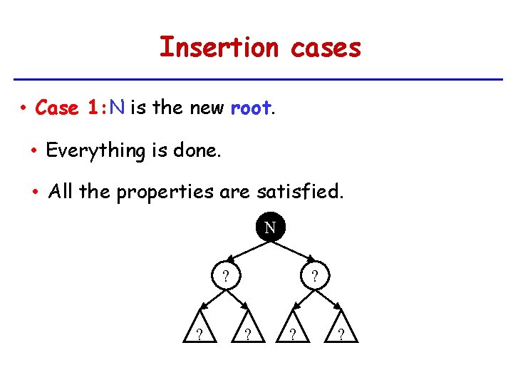
Insertion cases • Case 1: N is the new root. • Everything is done. • All the properties are satisfied. N ? ? ? ?

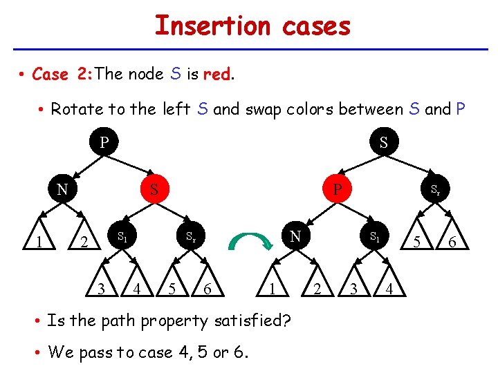
Insertion cases • Case 2: The node S is red. • Rotate to the left S and swap colors between S and P P S N 1 P S Sl 2 3 N Sr 4 5 Sr 6 1 • Is the path property satisfied? • We pass to case 4, 5 or 6. Sl 2 3 5 4 6

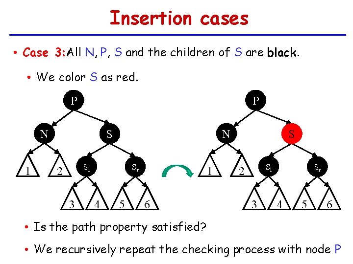
Insertion cases • Case 3: All N, P, S and the children of S are black. • We color S as red. P P N 1 N S Sl 2 3 Sr 4 5 1 6 S Sl 2 3 Sr 4 5 6 • Is the path property satisfied? • We recursively repeat the checking process with node P

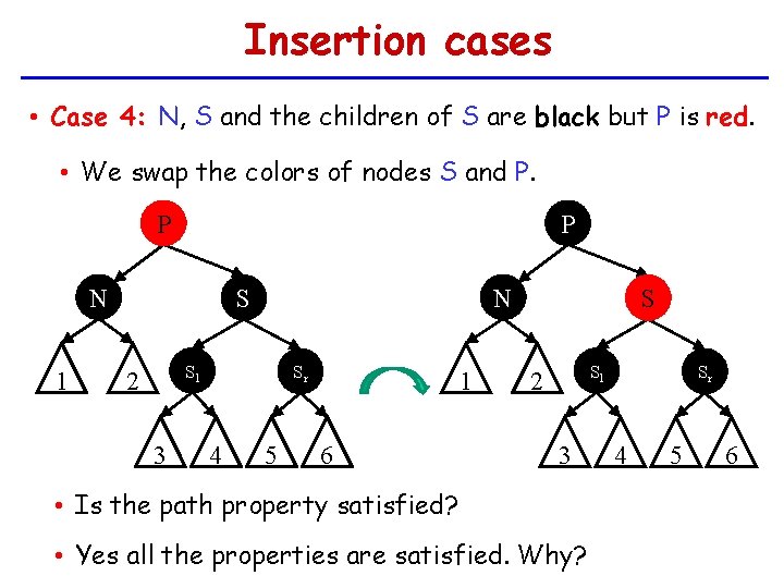
Insertion cases • Case 4: N, S and the children of S are black but P is red. • We swap the colors of nodes S and P. P P N 1 N S Sl 2 3 Sr 4 5 1 6 S Sl 2 3 • Is the path property satisfied? • Yes all the properties are satisfied. Why? Sr 4 5 6

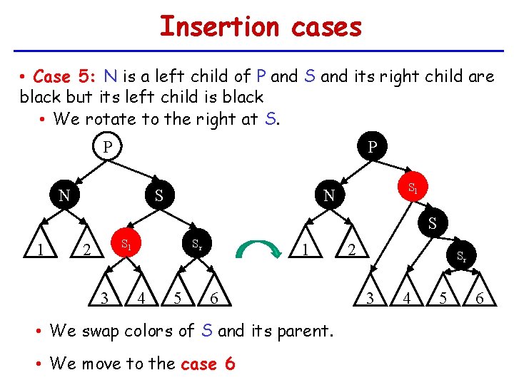
Insertion cases • Case 5: N is a left child of P and S and its right child are black but its left child is black • We rotate to the right at S. P P N Sl N S S 1 Sl 2 3 Sr 4 5 1 6 • We swap colors of S and its parent. • We move to the case 6 2 Sr 3 4 5 6

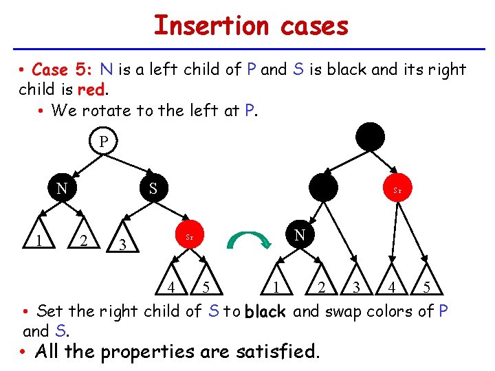
Insertion cases • Case 5: N is a left child of P and S is black and its right child is red. • We rotate to the left at P. S P N 1 P S 2 3 Sr Sr N 4 5 3 4 5 1 2 • Set the right child of S to black and swap colors of P and S. • All the properties are satisfied.

Summary − Key point: there exist data structures (2 -4 trees and red-black trees) that support Sorted. Set operations in O(log n) worst-case time per operation − Implementation difficulty is considerably higher than Scapegoat trees/skiplists/treaps − Look more closely at add. Fixup(u) and remove. Fixup(u) − Amortized analysis shows that they do only O(1) work on average

Summary − Key point: there exist data structures (2 -4 trees and red-black trees) that support Sorted. Set operations in O(log n) worst-case time per operation − Theorem: Starting with an empty red-black tree, any sequence of m add(x)/remove(x) operations performs only O(m) rotations and color changes − This is useful if want to apply persistence to remember old versions of the tree for later use

Summary − Skiplists: find(x)/add(x)/remove(x) in O(log n) expected time per operation. − Treaps: find(x)/add(x)/remove(x) in O(log n) expected time per operation. − Scapegoat trees: find(x) in O(log n) worst-case time per operation, add(x)/remove(x) in O(log n) amortized time per operation. − Red-black trees: find(x)/add(x)/remove(x) in O(log n) worst-case time per operation − All structures, except scapegoat trees do O(1) amortized (or expected) restructuring per add(x)/remove(x) operation