Outline Recap camera calibration Epipolar Geometry Oriented and

Outline • Recap camera calibration • Epipolar Geometry

Oriented and Translated Camera R jw t kw Ow iw

Degrees of freedom 5 6

How to calibrate the camera?

How do we calibrate a camera? 880 43 270 886 745 943 476 419 317 783 235 665 655 427 412 746 434 525 716 602 214 203 197 347 302 128 590 214 335 521 427 429 362 333 415 351 415 234 308 187 312. 747 309. 140 30. 086 305. 796 311. 649 30. 356 307. 694 312. 358 30. 418 310. 149 307. 186 29. 298 311. 937 310. 105 29. 216 311. 202 307. 572 30. 682 307. 106 306. 876 28. 660 309. 317 312. 490 30. 230 307. 435 310. 151 29. 318 308. 253 306. 300 28. 881 306. 650 309. 301 28. 905 308. 069 306. 831 29. 189 309. 671 308. 834 29. 029 308. 255 309. 955 29. 267 307. 546 308. 613 28. 963 311. 036 309. 206 28. 913 307. 518 308. 175 29. 069 309. 950 311. 262 29. 990 312. 160 310. 772 29. 080 311. 988 312. 709 30. 514

Method 1 – homogeneous linear system • Solve for m’s entries using linear least squares Ax=0 form [U, S, V] = svd(A); M = V(: , end); M = reshape(M, [], 3)';

For project 3, we want the camera center

Estimate of camera center 1. 0486 -1. 6851 -0. 9437 1. 0682 0. 6077 1. 2543 -0. 2709 -0. 4571 -0. 7902 0. 7318 -1. 0580 0. 3464 0. 3137 -0. 4310 -0. 4799 0. 6109 -0. 4081 -0. 1109 0. 5129 0. 1406 -0. 3645 -0. 4004 -0. 4200 0. 0699 -0. 0771 -0. 6454 0. 8635 -0. 3645 0. 0307 0. 6382 0. 3312 0. 3377 0. 1189 0. 0242 0. 2920 0. 0830 0. 2920 -0. 2992 -0. 0575 -0. 4527 1. 5706 -1. 5282 -0. 6821 0. 4124 1. 2095 0. 8819 -0. 9442 0. 0415 -0. 7975 -0. 4329 -1. 1475 -0. 5149 0. 1993 -0. 4320 -0. 7481 0. 8078 -0. 7605 0. 3237 1. 3089 1. 2323 -0. 1490 0. 9695 1. 2856 -1. 0201 0. 2812 -0. 8481 -1. 1583 1. 3445 0. 3017 -1. 4151 -0. 0772 -1. 1784 -0. 2854 0. 2143 -0. 3840 -0. 1196 -0. 5792 0. 7970 0. 5786 1. 4421 0. 2598 0. 3802 0. 4078 -0. 0915 -0. 1280 0. 5255 -0. 3759 0. 3240 -0. 0826 -0. 2774 -0. 2667 -0. 1401 -0. 2114 -0. 1053 -0. 2408 -0. 2631 -0. 1936 0. 2170 -0. 1887 0. 4506

Oriented and Translated Camera R jw t kw Ow iw

Recovering the camera center This is not the camera center C. It is –RC (because a point will be rotated before tx, ty, and tz are added) So we need -R-1 K-1 m 4 to get C This is t * K So K-1 m 4 is t Q is K * R. So we just need -Q-1 m 4 Q

Estimate of camera center 1. 0486 -1. 6851 -0. 9437 1. 0682 0. 6077 1. 2543 -0. 2709 -0. 4571 -0. 7902 0. 7318 -1. 0580 0. 3464 0. 3137 -0. 4310 -0. 4799 0. 6109 -0. 4081 -0. 1109 0. 5129 0. 1406 -0. 3645 -0. 4004 -0. 4200 0. 0699 -0. 0771 -0. 6454 0. 8635 -0. 3645 0. 0307 0. 6382 0. 3312 0. 3377 0. 1189 0. 0242 0. 2920 0. 0830 0. 2920 -0. 2992 -0. 0575 -0. 4527 1. 5706 -1. 5282 -0. 6821 0. 4124 1. 2095 0. 8819 -0. 9442 0. 0415 -0. 7975 -0. 4329 -1. 1475 -0. 5149 0. 1993 -0. 4320 -0. 7481 0. 8078 -0. 7605 0. 3237 1. 3089 1. 2323 -0. 1490 0. 9695 1. 2856 -1. 0201 0. 2812 -0. 8481 -1. 1583 1. 3445 0. 3017 -1. 4151 -0. 0772 -1. 1784 -0. 2854 0. 2143 -0. 3840 -0. 1196 -0. 5792 0. 7970 0. 5786 1. 4421 0. 2598 0. 3802 0. 4078 -0. 0915 -0. 1280 0. 5255 -0. 3759 0. 3240 -0. 0826 -0. 2774 -0. 2667 -0. 1401 -0. 2114 -0. 1053 -0. 2408 -0. 2631 -0. 1936 0. 2170 -0. 1887 0. 4506

Epipolar Geometry and Stereo Vision Chapter 7. 2 in Szeliski Many slides adapted from Derek Hoiem, Lana Lazebnik, Silvio Saverese, Steve Seitz, many figures from Hartley & Zisserman

• Epipolar geometry – Relates cameras from two positions

Depth from Stereo • Goal: recover depth by finding image coordinate x’ that corresponds to x X X z x x x' x’ f C f Baseline B C’

Depth from Stereo • Goal: recover depth by finding image coordinate x’ that corresponds to x • Sub-Problems 1. Calibration: How do we recover the relation of the cameras (if not already known)? 2. Correspondence: How do we search for the matching point x’? X x x'

Correspondence Problem x ? • We have two images taken from cameras with different intrinsic and extrinsic parameters • How do we match a point in the first image to a point in the second? How can we constrain our search?

Where do we need to search?

Key idea: Epipolar constraint

Key idea: Epipolar constraint X X X x x’ x’ x’ Potential matches for x have to lie on the corresponding line l’. Potential matches for x’ have to lie on the corresponding line l.

Wouldn’t it be nice to know where matches can live? To constrain our 2 d search to 1 d.

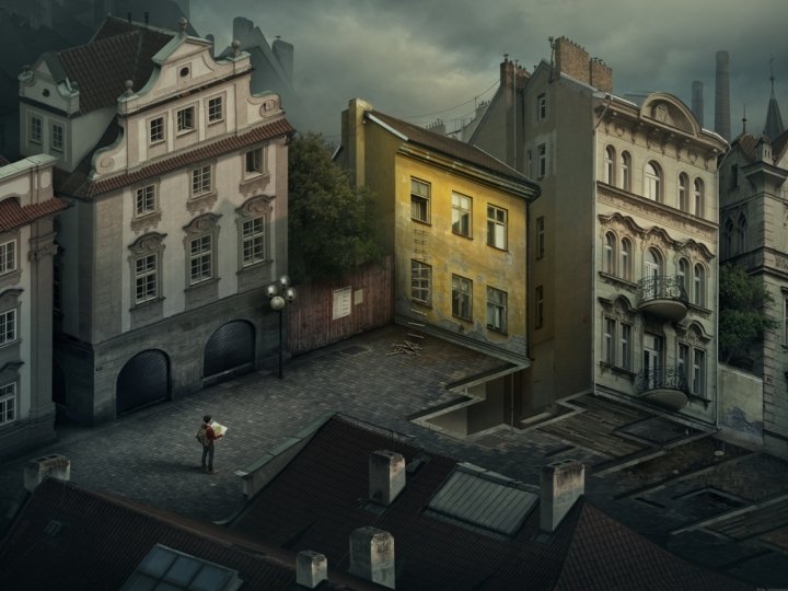
VLFeat’s 800 most confident matches among 10, 000+ local features.

Epipolar geometry: notation X x x’ • Baseline – line connecting the two camera centers • Epipoles = intersections of baseline with image planes = projections of the other camera center • Epipolar Plane – plane containing baseline (1 D family)

Epipolar geometry: notation X x x’ • Baseline – line connecting the two camera centers • Epipoles = intersections of baseline with image planes = projections of the other camera center • Epipolar Plane – plane containing baseline (1 D family) • Epipolar Lines - intersections of epipolar plane with image planes (always come in corresponding pairs)

Example: Converging cameras

Example: Motion parallel to image plane

Example: Forward motion What would the epipolar lines look like if the camera moves directly forward?

Example: Forward motion e’ e Epipole has same coordinates in both images. Points move along lines radiating from e: “Focus of expansion”

Epipolar constraint: Calibrated case X x x’
")
Essential matrix X x x’ Essential Matrix (Longuet-Higgins, 1981)

The Fundamental Matrix Without knowing K and K’, we can define a similar relation using unknown normalized coordinates Fundamental Matrix (Faugeras and Luong, 1992)

Properties of the Fundamental matrix X x • • • x’ F x’ = 0 is the epipolar line associated with x’ FTx = 0 is the epipolar line associated with x F e’ = 0 and FTe = 0 F is singular (rank two): det(F)=0 F has seven degrees of freedom: 9 entries but defined up to scale, det(F)=0

Estimating the Fundamental Matrix • 8 -point algorithm – Least squares solution using SVD on equations from 8 pairs of correspondences – Enforce det(F)=0 constraint using SVD on F • 7 -point algorithm – Use least squares to solve for null space (two vectors) using SVD and 7 pairs of correspondences – Solve for linear combination of null space vectors that satisfies det(F)=0 • Minimize reprojection error – Non-linear least squares Note: estimation of F (or E) is degenerate for a planar scene.

8 -point algorithm 1. Solve a system of homogeneous linear equations a. Write down the system of equations

8 -point algorithm 1. Solve a system of homogeneous linear equations a. Write down the system of equations b. Solve f from Af=0 using SVD Matlab: [U, S, V] = svd(A); f = V(: , end); F = reshape(f, [3 3])’;

Need to enforce singularity constraint

8 -point algorithm 1. Solve a system of homogeneous linear equations a. Write down the system of equations b. Solve f from Af=0 using SVD Matlab: [U, S, V] = svd(A); f = V(: , end); F = reshape(f, [3 3])’; 2. Resolve det(F) = 0 constraint using SVD Matlab: [U, S, V] = svd(F); S(3, 3) = 0; F = U*S*V’;

8 -point algorithm 1. Solve a system of homogeneous linear equations a. Write down the system of equations b. Solve f from Af=0 using SVD 2. Resolve det(F) = 0 constraint by SVD Notes: • Use RANSAC to deal with outliers (sample 8 points) – How to test for outliers?

Problem with eight-point algorithm

Problem with eight-point algorithm Poor numerical conditioning Can be fixed by rescaling the data
 • Center the image data at the origin,")
The normalized eight-point algorithm (Hartley, 1995) • Center the image data at the origin, and scale it so the mean squared distance between the origin and the data points is 2 pixels • Use the eight-point algorithm to compute F from the normalized points • Enforce the rank-2 constraint (for example, take SVD of F and throw out the smallest singular value) • Transform fundamental matrix back to original units: if T and T’ are the normalizing transformations in the two images, than the fundamental matrix in original coordinates is T’T F T

VLFeat’s 800 most confident matches among 10, 000+ local features.

Epipolar lines

Keep only the matches at are “inliers” with respect to the “best” fundamental matrix
- Slides: 45