Outline Multi period stochastic Inventory control Continuous review

Outline • Multi period stochastic Inventory control – Continuous review • (Q, R) model • Service level; Cycle service level and Fill rate – Periodic Review • Order-up-to policy • (s, S) policy • Single period stochastic inventory control – Newsboy model • ABC analysis for multi item inventory control

Sources of uncertainity – Demand • Could be correlated or independent across time, across several items. • Could be stationary or nonstationary (trend, seasonality) • We will assume single item, demand of the item is stationary, and independenly identically distributed across time. – Lead time – Product quality

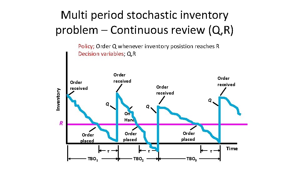
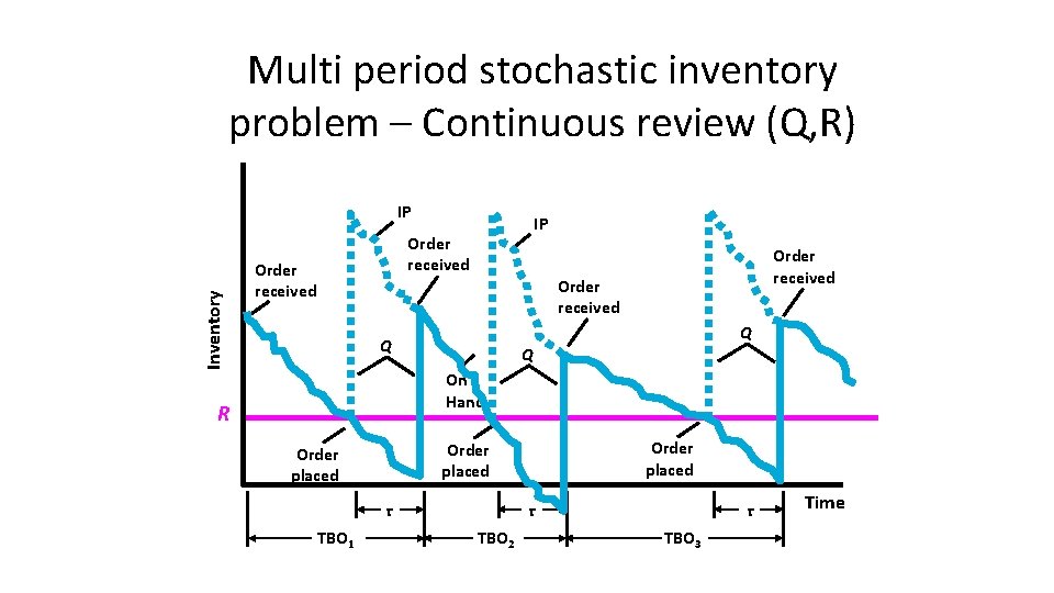
Multi period stochastic inventory problem – Continuous review (Q, R) Inventory Policy; Order Q whenever inventory posistion reaches R Decision variables; Q, R Order received Q Q Q On Hand R τ TBO 1 Order placed τ TBO 2 τ TBO 3 Time

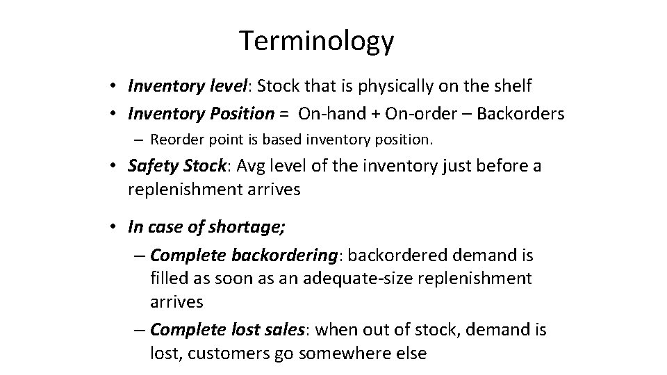
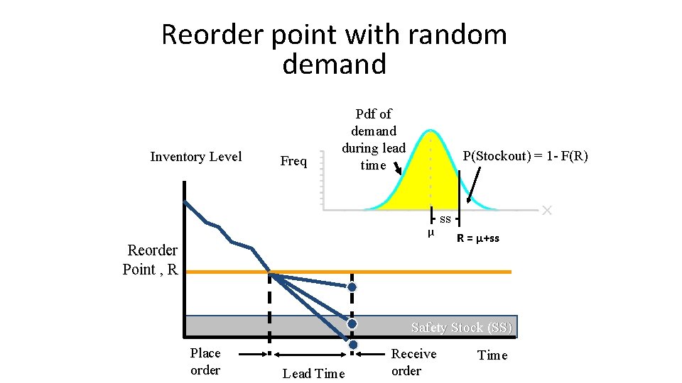
Terminology • Inventory level: Stock that is physically on the shelf • Inventory Position = On-hand + On-order – Backorders – Reorder point is based inventory position. • Safety Stock: Avg level of the inventory just before a replenishment arrives • In case of shortage; – Complete backordering: backordered demand is filled as soon as an adequate-size replenishment arrives – Complete lost sales: when out of stock, demand is lost, customers go somewhere else

Multi period stochastic inventory problem – Continuous review (Q, R) Inventory IP IP Order received Q Q Q On Hand R τ TBO 1 Order placed τ TBO 2 τ TBO 3 Time

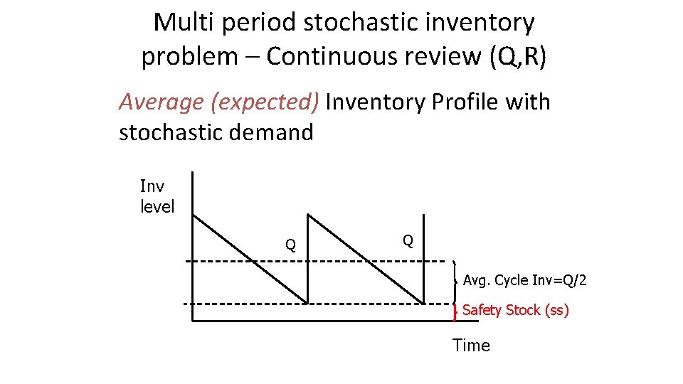
Multi period stochastic inventory problem – Continuous review (Q, R) Average (expected) Inventory Profile with stochastic demand Inv level Q Q Avg. Cycle Inv=Q/2 Safety Stock (ss) Time

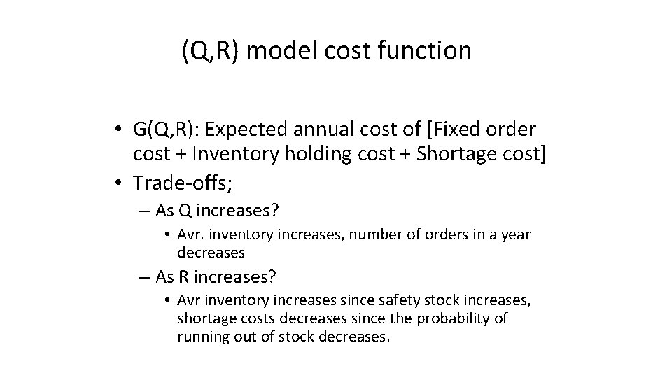
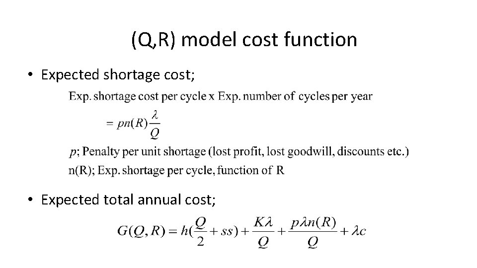
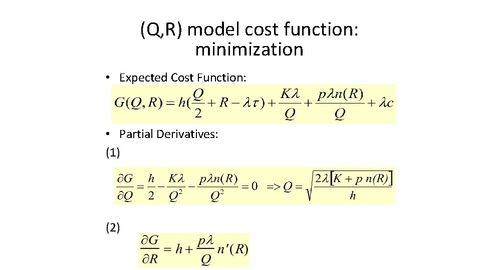
(Q, R) model cost function • G(Q, R): Expected annual cost of [Fixed order cost + Inventory holding cost + Shortage cost] • Trade-offs; – As Q increases? • Avr. inventory increases, number of orders in a year decreases – As R increases? • Avr inventory increases since safety stock increases, shortage costs decreases since the probability of running out of stock decreases.

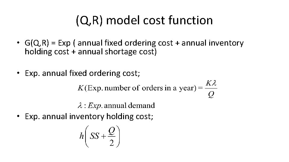
(Q, R) model cost function • G(Q, R) = Exp ( annual fixed ordering cost + annual inventory holding cost + annual shortage cost) • Exp. annual fixed ordering cost; • Exp. annual inventory holding cost;

(Q, R) model cost function • Expected shortage cost; • Expected total annual cost;

Reorder point with random demand Inventory Level Freq Pdf of demand during lead time P(Stockout) = 1 - F(R) μ Reorder Point , R ss R = μ+ss Safety Stock (SS) Place order Lead Time Receive order Time

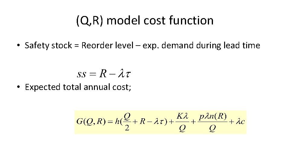
(Q, R) model cost function • Safety stock = Reorder level – exp. demand during lead time • Expected total annual cost;

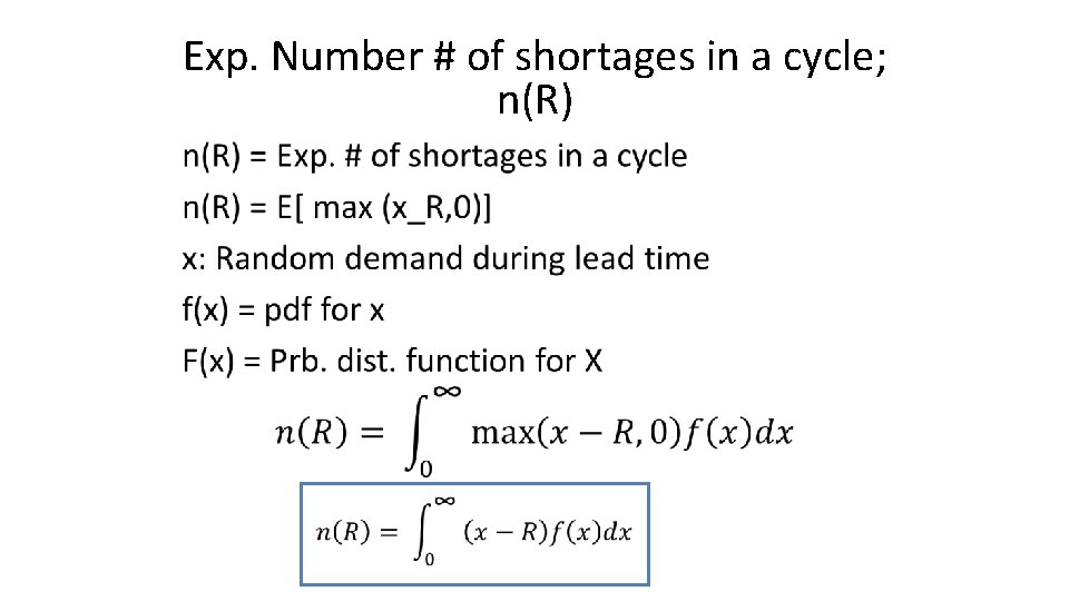
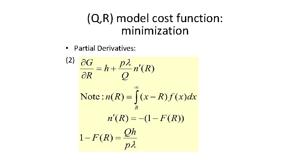
Exp. Number # of shortages in a cycle; n(R) •

(Q, R) model cost function: minimization • Expected Cost Function: • Partial Derivatives: (1) (2)

(Q, R) model cost function: minimization • Partial Derivatives: (2)

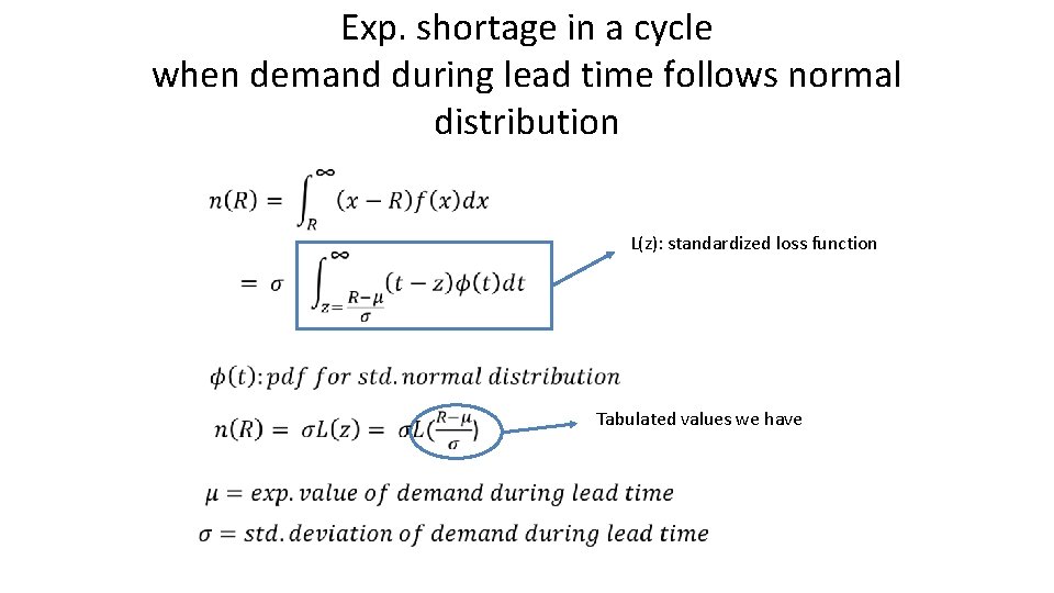
Exp. shortage in a cycle when demand during lead time follows normal distribution L(z): standardized loss function Tabulated values we have

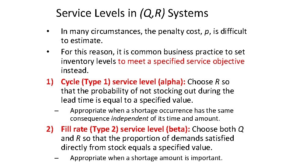
Service Levels in (Q, R) Systems In many circumstances, the penalty cost, p, is difficult to estimate. • For this reason, it is common business practice to set inventory levels to meet a specified service objective instead. 1) Cycle (Type 1) service level (alpha): Choose R so that the probability of not stocking out during the lead time is equal to a specified value. • – Appropriate when a shortage occurrence has the same consequence independent of its time and amount. 2) Fill rate (Type 2) service level (beta): Choose both Q and R so that the proportion of demands satisfied directly from stock equals a specified value. – Appropriate when a shortage amount is important.

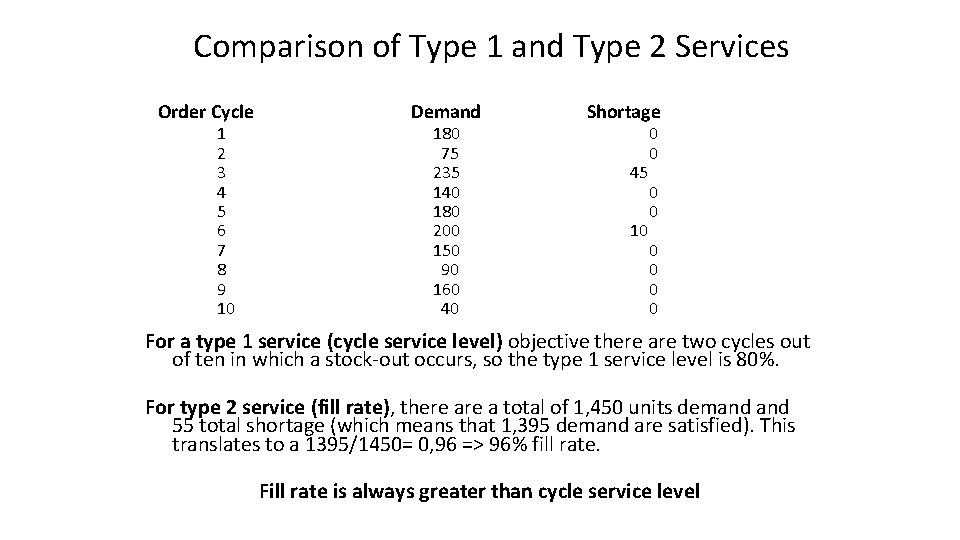
Comparison of Type 1 and Type 2 Services Order Cycle 1 2 3 4 5 6 7 8 9 10 Demand 180 75 235 140 180 200 150 90 160 40 Shortage 45 10 0 0 0 0 For a type 1 service (cycle service level) objective there are two cycles out of ten in which a stock-out occurs, so the type 1 service level is 80%. For type 2 service (fill rate), there a total of 1, 450 units demand 55 total shortage (which means that 1, 395 demand are satisfied). This translates to a 1395/1450= 0, 96 => 96% fill rate. Fill rate is always greater than cycle service level

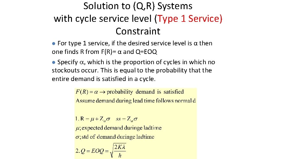
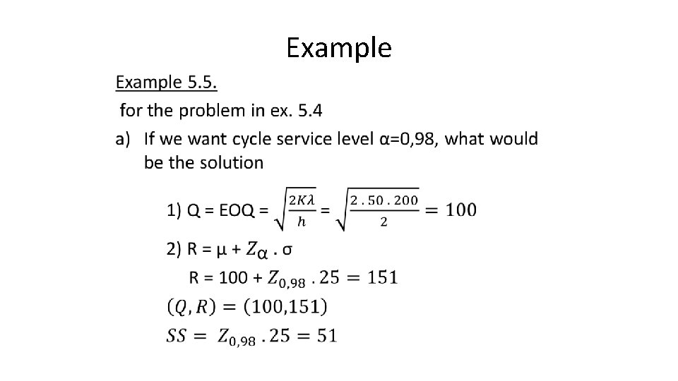
Solution to (Q, R) Systems with cycle service level (Type 1 Service) Constraint l For type 1 service, if the desired service level is α then one finds R from F(R)= α and Q=EOQ l Specify a, which is the proportion of cycles in which no stockouts occur. This is equal to the probability that the entire demand is satisfied in a cycle.

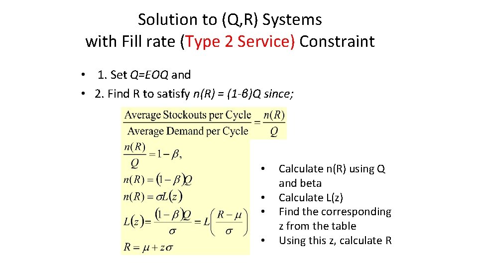
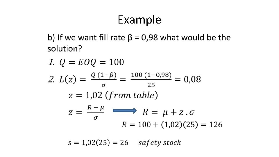
Solution to (Q, R) Systems with Fill rate (Type 2 Service) Constraint • 1. Set Q=EOQ and • 2. Find R to satisfy n(R) = (1 -β)Q since; • • Calculate n(R) using Q and beta Calculate L(z) Find the corresponding z from the table Using this z, calculate R

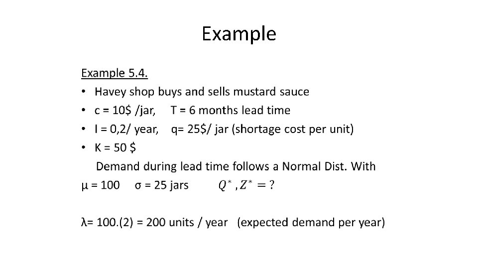
Example •

Example •

Example •

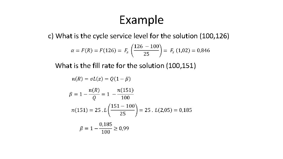
Example c) What is the cycle service level for the solution (100, 126) What is the fill rate for the solution (100, 151)

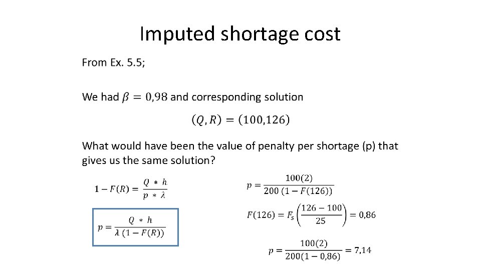
Imputed shortage cost •

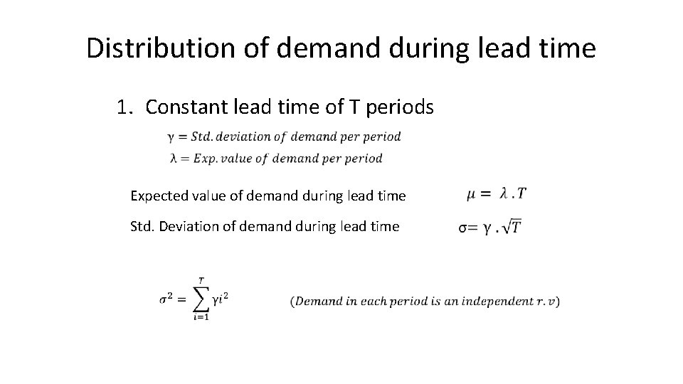
Distribution of demand during lead time 1. Constant lead time of T periods Expected value of demand during lead time Std. Deviation of demand during lead time

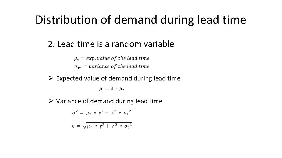
Distribution of demand during lead time 2. Lead time is a random variable Ø Expected value of demand during lead time Ø Variance of demand during lead time

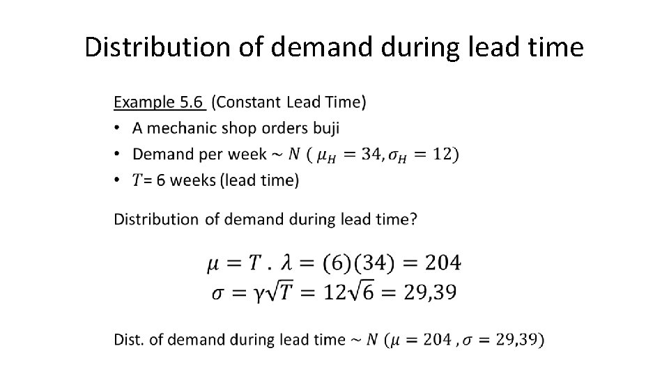
Distribution of demand during lead time •

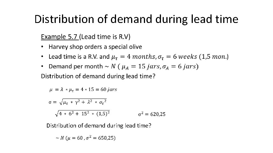
Distribution of demand during lead time • Distribution of demand during lead time?