Outline Logistics Bayes Nets joint probability distribution conditional

Outline • Logistics • Bayes Nets – joint probability distribution, conditional independence – graphical representation – inference (deduction & diagnosis) • Review
Logistics • Learning Problem Set Due • Project Status – Movie Ids – Sample Queries • Reports Due 6/11
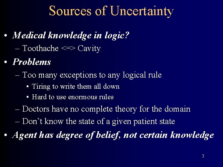
Sources of Uncertainty • Medical knowledge in logic? – Toothache <=> Cavity • Problems – Too many exceptions to any logical rule • Tiring to write them all down • Hard to use enormous rules – Doctors have no complete theory for the domain – Don’t know the state of a given patient state • Agent has degree of belief, not certain knowledge 3
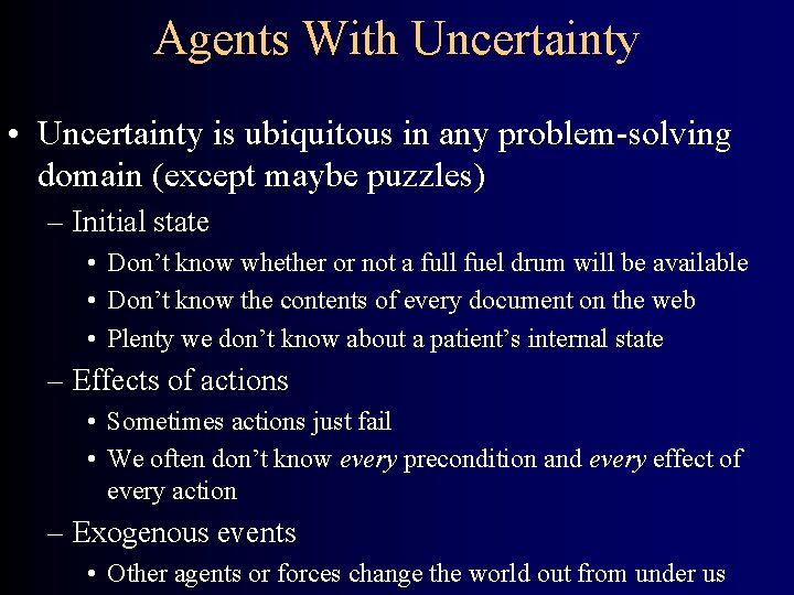
Agents With Uncertainty • Uncertainty is ubiquitous in any problem-solving domain (except maybe puzzles) – Initial state • Don’t know whether or not a full fuel drum will be available • Don’t know the contents of every document on the web • Plenty we don’t know about a patient’s internal state – Effects of actions • Sometimes actions just fail • We often don’t know every precondition and every effect of every action – Exogenous events • Other agents or forces change the world out from under us
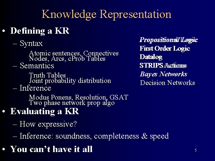
Knowledge Representation • Defining a KR – Syntax Atomic sentences, Connectives Nodes, Arcs, c. Prob Tables – Semantics Truth Tables Joint probability distribution – Inference Propositional Logic First Order Logic Datalog STRIPSActions Bayes Networks Decision Networks Modus Ponens, Resolution, GSAT Two phase network prop algo • Evaluating a KR – How expressive? – Inference: soundness, completeness & speed • You can’t have it all 5
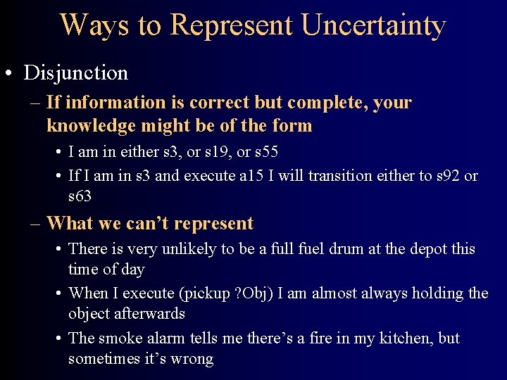
Ways to Represent Uncertainty • Disjunction – If information is correct but complete, your knowledge might be of the form • I am in either s 3, or s 19, or s 55 • If I am in s 3 and execute a 15 I will transition either to s 92 or s 63 – What we can’t represent • There is very unlikely to be a full fuel drum at the depot this time of day • When I execute (pickup ? Obj) I am almost always holding the object afterwards • The smoke alarm tells me there’s a fire in my kitchen, but sometimes it’s wrong
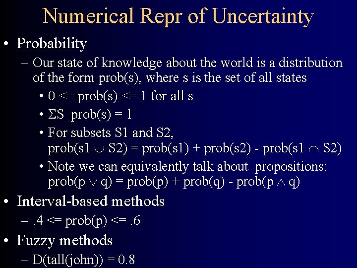
Numerical Repr of Uncertainty • Probability – Our state of knowledge about the world is a distribution of the form prob(s), where s is the set of all states • 0 <= prob(s) <= 1 for all s • S prob(s) = 1 • For subsets S 1 and S 2, prob(s 1 S 2) = prob(s 1) + prob(s 2) - prob(s 1 S 2) • Note we can equivalently talk about propositions: prob(p q) = prob(p) + prob(q) - prob(p q) • Interval-based methods –. 4 <= prob(p) <=. 6 • Fuzzy methods – D(tall(john)) = 0. 8
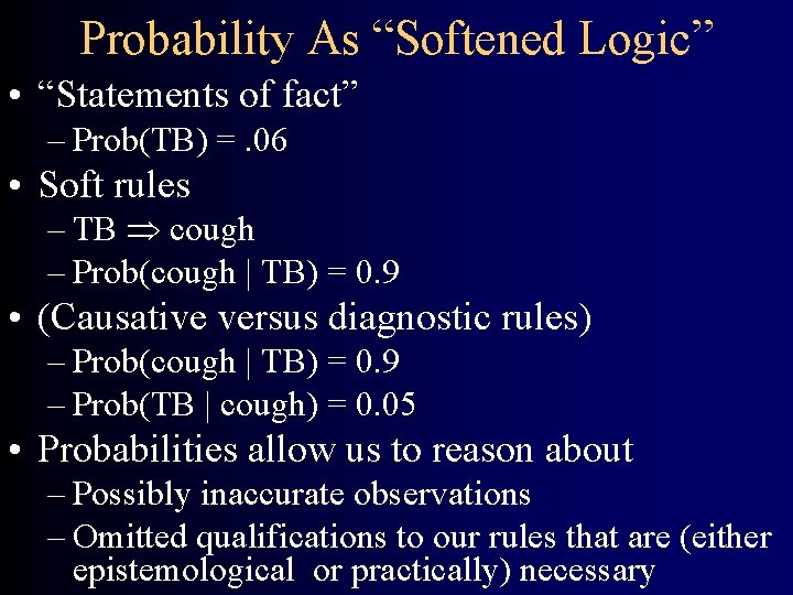
Probability As “Softened Logic” • “Statements of fact” – Prob(TB) =. 06 • Soft rules – TB cough – Prob(cough | TB) = 0. 9 • (Causative versus diagnostic rules) – Prob(cough | TB) = 0. 9 – Prob(TB | cough) = 0. 05 • Probabilities allow us to reason about – Possibly inaccurate observations – Omitted qualifications to our rules that are (either epistemological or practically) necessary
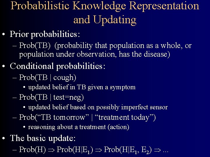
Probabilistic Knowledge Representation and Updating • Prior probabilities: – Prob(TB) (probability that population as a whole, or population under observation, has the disease) • Conditional probabilities: – Prob(TB | cough) • updated belief in TB given a symptom – Prob(TB | test=neg) • updated belief based on possibly imperfect sensor – Prob(“TB tomorrow” | “treatment today”) • reasoning about a treatment (action) • The basic update: – Prob(H) Prob(H|E 1, E 2) . . .
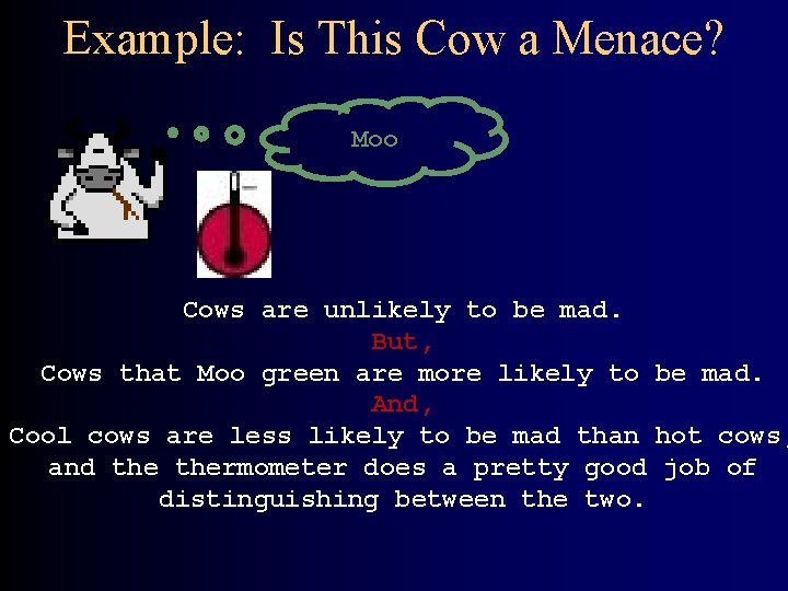
Example: Is This Cow a Menace? Moo Cows are unlikely to be mad. But, Cows that Moo green are more likely to be mad. And, Cool cows are less likely to be mad than hot cows, and thermometer does a pretty good job of distinguishing between the two.
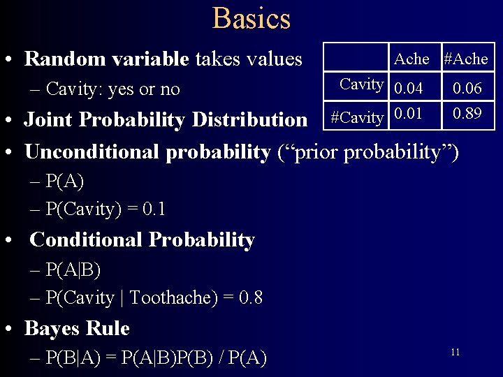
Basics • Random variable takes values – Cavity: yes or no Ache #Ache Cavity 0. 04 #Cavity 0. 01 0. 06 0. 89 • Joint Probability Distribution • Unconditional probability (“prior probability”) – P(A) – P(Cavity) = 0. 1 • Conditional Probability – P(A|B) – P(Cavity | Toothache) = 0. 8 • Bayes Rule – P(B|A) = P(A|B)P(B) / P(A) 11
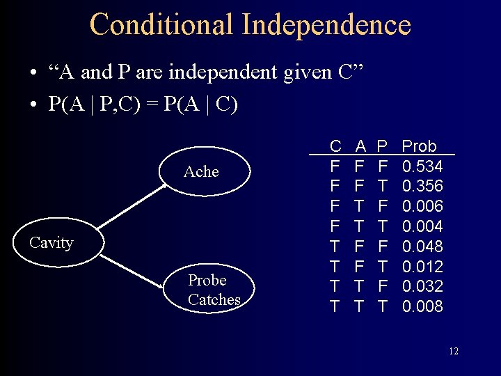
Conditional Independence • “A and P are independent given C” • P(A | P, C) = P(A | C) Ache Cavity Probe Catches C F F T T A F F T T P F T F T Prob 0. 534 0. 356 0. 004 0. 048 0. 012 0. 032 0. 008 12
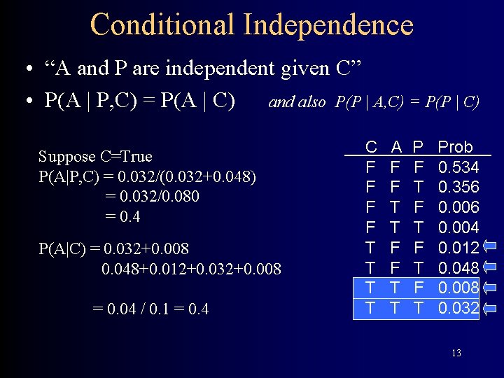
Conditional Independence • “A and P are independent given C” • P(A | P, C) = P(A | C) and also P(P | A, C) = P(P | C) Suppose C=True P(A|P, C) = 0. 032/(0. 032+0. 048) = 0. 032/0. 080 = 0. 4 P(A|C) = 0. 032+0. 008 0. 048+0. 012+0. 032+0. 008 = 0. 04 / 0. 1 = 0. 4 C F F T T A F F T T P F T F T Prob 0. 534 0. 356 0. 004 0. 012 0. 048 0. 008 0. 032 13

Conditional Independence • Can encode joint probability distribution in compact form Ache C T F P(A) 0. 4 0. 02 C T F P(P) 0. 8 0. 4 Cavity P(C). 01 Probe Catches C F F T T A F F T T P F T F T Prob 0. 534 0. 356 0. 004 0. 012 0. 048 0. 008 0. 032 14
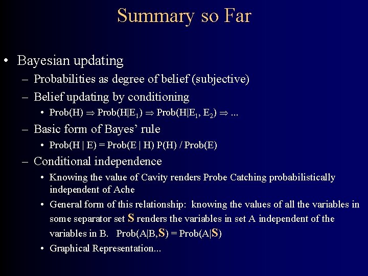
Summary so Far • Bayesian updating – Probabilities as degree of belief (subjective) – Belief updating by conditioning • Prob(H) Prob(H|E 1, E 2) . . . – Basic form of Bayes’ rule • Prob(H | E) = Prob(E | H) P(H) / Prob(E) – Conditional independence • Knowing the value of Cavity renders Probe Catching probabilistically independent of Ache • General form of this relationship: knowing the values of all the variables in some separator set S renders the variables in set A independent of the variables in B. Prob(A|B, S) = Prob(A|S) • Graphical Representation. . .
Computational Models for Probabilistic Reasoning • What we want – a “probabilistic knowledge base” where domain knowledge is represented by propositions, unconditional, and conditional probabilities – an inference engine that will compute Prob(formula | “all evidence collected so far”) • Problems – elicitation: what parameters do we need to ensure a complete and consistent knowledge base? – computation: how do we compute the probabilities efficiently? • Answer (to both problems) – a representation that makes structure (dependencies and independencies) explicit
Causality • Probability theory represents correlation – Absolutely no notion of causality – Smoking and cancer are correlated • Bayes nets use directed arcs to represent causality – Write only (significant) direct causal effects – Can lead to much smaller encoding than full JPD – Many Bayes nets correspond to the same JPD – Some may be simpler than others 17
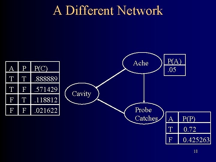
A Different Network A T T F F P T F P(C). 888889. 571429. 118812. 021622 Ache P(A). 05 Cavity Probe Catches A T F P(P) 0. 72 0. 425263 18
Creating a Network • 1: Bayes net = representation of a JPD • 2: Bayes net = set of cond. independence statements • If create correct structure • Ie one representing causlity – Then get a good network • I. e. one that’s small = easy to compute with • One that is easy to fill in numbers 19
Example My house alarm system just sounded (A). Both an earthquake (E) and a burglary (B) could set it off. John will probably hear the alarm; if so he’ll call (J). But sometimes John calls even when the alarm is silent Mary might hear the alarm and call too (M), but not as reliably We could be assured a complete and consistent model by fully specifying the joint distribution: Prob(A, E, B, J, M) Prob(A, E, B, J, ~M) etc.
Structural Models Instead of starting with numbers, we will start with structural relationships among the variables direct causal relationship from Earthquake to Radio direct causal relationship from Burglar to Alarm direct causal relationship from Alarm to John. Call Earthquake and Burglar tend to occur independently etc.
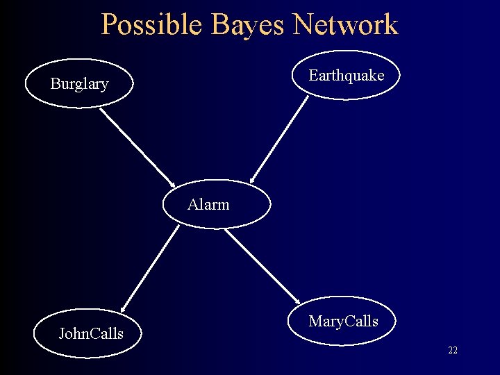
Possible Bayes Network Earthquake Burglary Alarm John. Calls Mary. Calls 22
Graphical Models and Problem Parameters • What probabilities need I specify to ensure a complete, consistent model given – the variables I have identified – the dependence and independence relationships I have specified by building a graph structure • Answer – provide an unconditional (prior) probability for every node in the graph with no parents – for all remaining, provide a conditional probability table • Prob(Child | Parent 1, Parent 2, Parent 3) for all possible combination of Parent 1, Parent 2, Parent 3 values

Complete Bayes Network Burglary Earthquake P(B). 001 Alarm John. Calls A T F P(J). 90. 05 B T T F F E T F P(E). 002 P(A). 95. 94. 29. 01 Mary. Calls A P(M) T. 70 F. 01 24
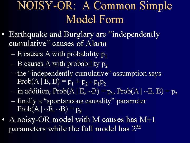
NOISY-OR: A Common Simple Model Form • Earthquake and Burglary are “independently cumulative” causes of Alarm – E causes A with probability p 1 – B causes A with probability p 2 – the “independently cumulative” assumption says Prob(A | E, B) = p 1 + p 2 - p 1 p 2 – in addition, Prob(A | E, ~B) = p 1, Prob(A | ~E, B) = p 2 – finally a “spontaneous causality” parameter Prob(A | ~E, ~B) = p 3 • A noisy-OR model with M causes has M+1 parameters while the full model has 2 M
More Complex Example My house alarm system just sounded (A). Both an earthquake (E) and a burglary (B) could set it off. Earthquakes tend to be reported on the radio (R). My neighbor will usually call me (N) if he (thinks he) sees a burglar. The police (P) sometimes respond when the alarm sounds. What structure is best?
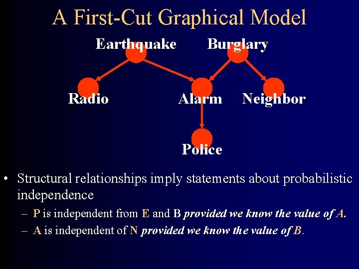
A First-Cut Graphical Model Earthquake Radio Burglary Alarm Neighbor Police • Structural relationships imply statements about probabilistic independence – P is independent from E and B provided we know the value of A. – A is independent of N provided we know the value of B.
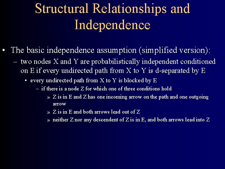
Structural Relationships and Independence • The basic independence assumption (simplified version): – two nodes X and Y are probabilistically independent conditioned on E if every undirected path from X to Y is d-separated by E • every undirected path from X to Y is blocked by E – if there is a node Z for which one of three conditions hold » Z is in E and Z has one incoming arrow on the path and one outgoing arrow » Z is in E and both arrows lead out of Z » neither Z nor any descendent of Z is in E, and both arrows lead into Z
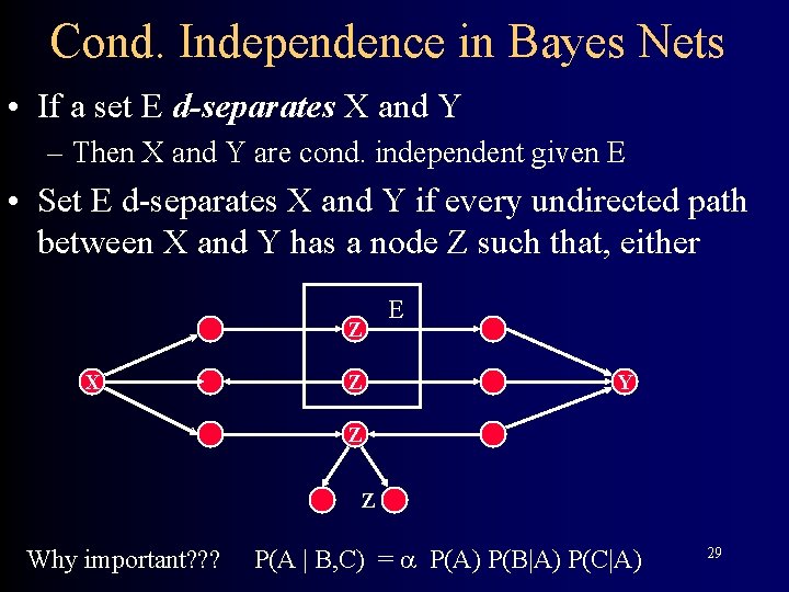
Cond. Independence in Bayes Nets • If a set E d-separates X and Y – Then X and Y are cond. independent given E • Set E d-separates X and Y if every undirected path between X and Y has a node Z such that, either Z X Z E Y Z Z Why important? ? ? P(A | B, C) = P(A) P(B|A) P(C|A) 29
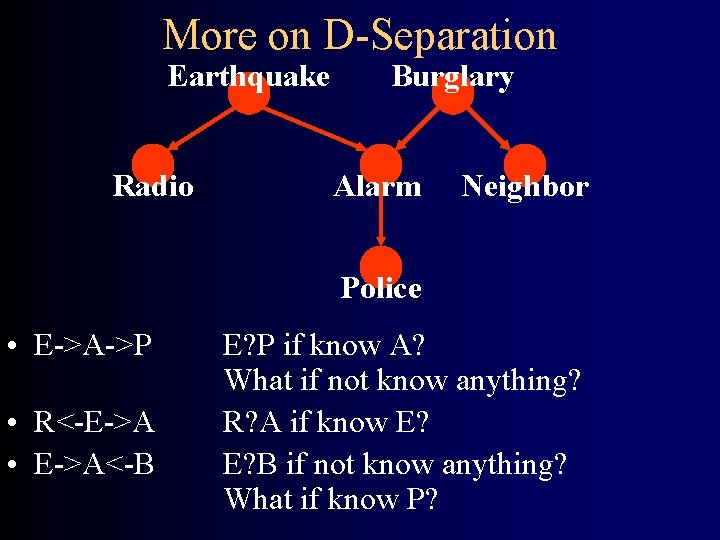
More on D-Separation Earthquake Radio Burglary Alarm Neighbor Police • E->A->P • R<-E->A • E->A<-B E? P if know A? What if not know anything? R? A if know E? E? B if not know anything? What if know P?
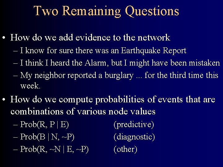
Two Remaining Questions • How do we add evidence to the network – I know for sure there was an Earthquake Report – I think I heard the Alarm, but I might have been mistaken – My neighbor reported a burglary. . . for the third time this week. • How do we compute probabilities of events that are combinations of various node values – Prob(R, P | E) – Prob(B | N, ~P) – Prob(R, ~N | E, ~P) (predictive) (diagnostic) (other)
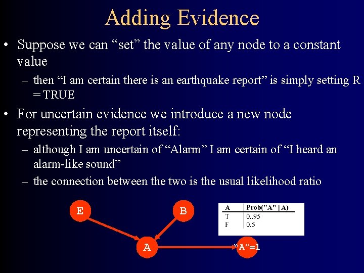
Adding Evidence • Suppose we can “set” the value of any node to a constant value – then “I am certain there is an earthquake report” is simply setting R = TRUE • For uncertain evidence we introduce a new node representing the report itself: – although I am uncertain of “Alarm” I am certain of “I heard an alarm-like sound” – the connection between the two is the usual likelihood ratio E B A “A”=1

Inference • Given exact values for evidence variables • Compute posterior probability of query variable P(B) Burglary. 001 Alarm Jon. Calls A P(J) T. 90 F. 05 Earthq B T T F F P(E). 002 E P(A) T. 95 F. 94 T. 29 F. 01 A P(M) Mary. Call T. 70 F. 01 • Diagnostic – effects to causes • Causal – causes to effects • Intercausal – between causes of common effect – explaining away • Mixed 33
Algorithm • In general: NP Complete • Easy for polytrees – I. e. only one undirected path between nodes • Express P(X|E) by – 1. Recursively passing support from ancestor down • “Causal support” – 2. Recursively calc contribution from descendants up • “Evidential support” • Speed: linear in the number of nodes (in polytree) 34
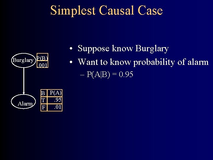
Simplest Causal Case Burglary P(B). 001 • Suppose know Burglary • Want to know probability of alarm – P(A|B) = 0. 95 Alarm B P(A). 95 T. 01 F
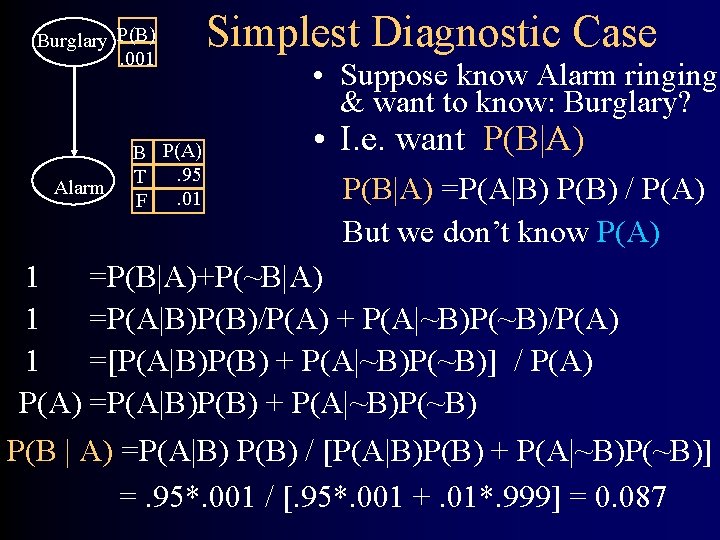
Burglary P(B). 001 Alarm B P(A). 95 T. 01 F Simplest Diagnostic Case • Suppose know Alarm ringing & want to know: Burglary? • I. e. want P(B|A) =P(A|B) P(B) / P(A) But we don’t know P(A) 1 =P(B|A)+P(~B|A) 1 =P(A|B)P(B)/P(A) + P(A|~B)P(~B)/P(A) 1 =[P(A|B)P(B) + P(A|~B)P(~B)] / P(A) =P(A|B)P(B) + P(A|~B)P(~B) P(B | A) =P(A|B) P(B) / [P(A|B)P(B) + P(A|~B)P(~B)] =. 95*. 001 / [. 95*. 001 +. 01*. 999] = 0. 087
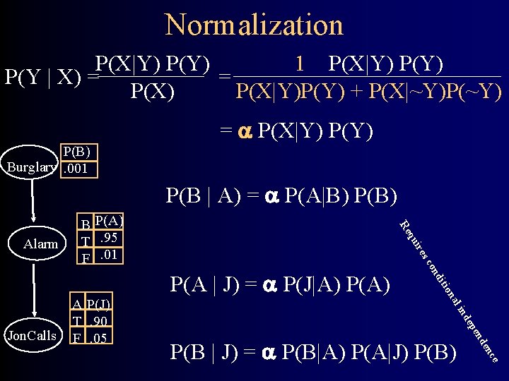
Normalization P(X|Y) P(Y) 1 P(X|Y) P(Y | X) = = P(X) P(X|Y)P(Y) + P(X|~Y)P(~Y) = P(X|Y) P(B) Burglary. 001 P(B | A) = P(A|B) P(B) es uir q Re Alarm B P(A) T. 95 F. 01 e nc de P(B | J) = P(B|A) P(A|J) P(B) n pe de l in na itio Jon. Calls A P(J) T. 90 F. 05 nd co P(A | J) = P(J|A) P(A)
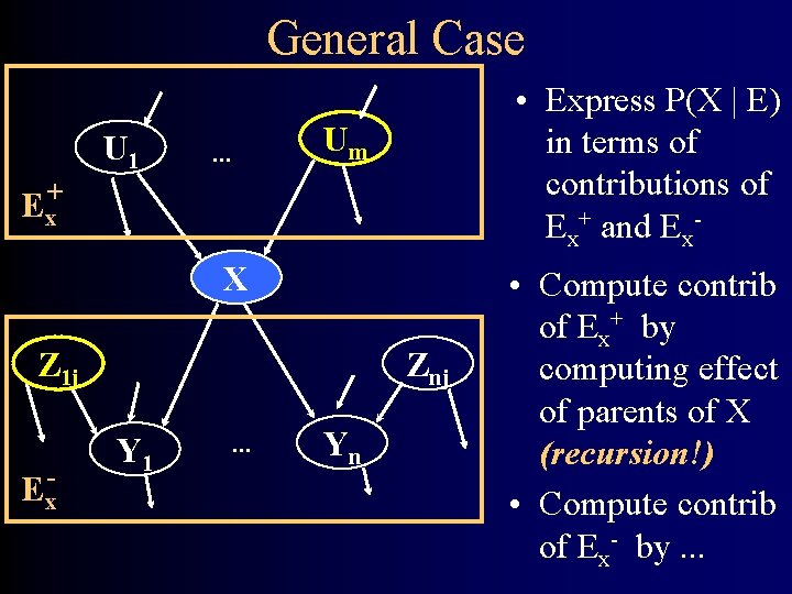
General Case U 1 • Express P(X | E) in terms of contributions of Ex+ and Ex- Um . . . + Ex X Z 1 j Ex- Znj Y 1 . . . Yn • Compute contrib of Ex+ by computing effect of parents of X (recursion!) • Compute contrib of Ex- by. . .
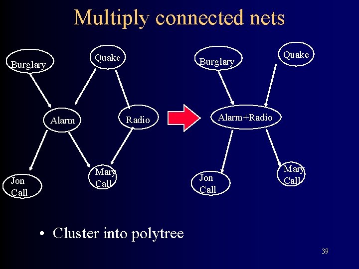
Multiply connected nets Quake Burglary Alarm+Radio Alarm Jon Call Burglary Mary Call Quake Jon Call Mary Call • Cluster into polytree 39
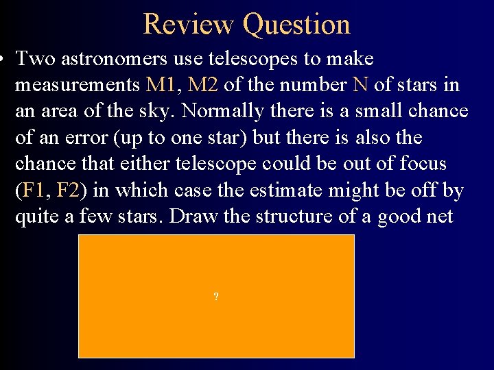
Review Question • Two astronomers use telescopes to make measurements M 1, M 2 of the number N of stars in an area of the sky. Normally there is a small chance of an error (up to one star) but there is also the chance that either telescope could be out of focus (F 1, F 2) in which case the estimate might be off by quite a few stars. Draw the structure of a good net F 1 F 2 N ? M 1 M 2
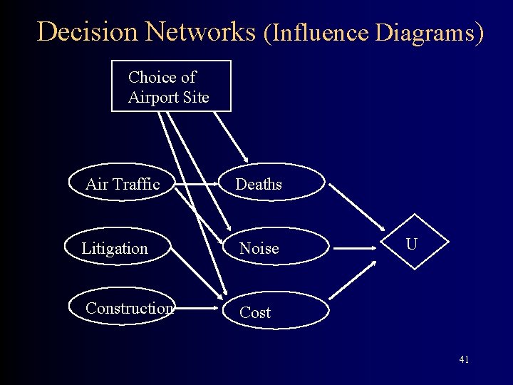
Decision Networks (Influence Diagrams) Choice of Airport Site Air Traffic Deaths Litigation Noise Construction Cost U 41
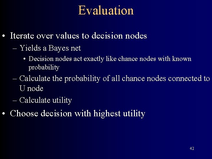
Evaluation • Iterate over values to decision nodes – Yields a Bayes net • Decision nodes act exactly like chance nodes with known probability – Calculate the probability of all chance nodes connected to U node – Calculate utility • Choose decision with highest utility 42
Outline • Logistics • Bayes Nets – joint probability distribution, conditional independence – graphical representation – inference (deduction & diagnosis) • Review
Course Topics by Week • • • Search & Constraint Satisfaction Knowledge Representation 1: Propositional Logic Autonomous Spacecraft 1: Configuration Mgmt Autonomous Spacecraft 2: Reactive Planning Information Integration 1: Knowledge Representation Information Integration 2: Planning • • Information Integration 3: Execution; Learning 1 Learn 2: Supervised Learning Learn 3: Wrapper Induction & Reinforcement Learn Bayes Nets: Representation & Inference
Unifying View of AI • Knowledge Representation – Expressiveness – Reasoning (Tractability) • Search – Space being searched – Algorithms & performance
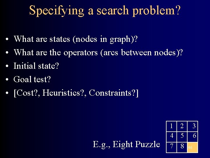
Specifying a search problem? • • • What are states (nodes in graph)? What are the operators (arcs between nodes)? Initial state? Goal test? [Cost? , Heuristics? , Constraints? ] E. g. , Eight Puzzle 1 2 4 5 7 8 3 6 46
Example: AI Planning • Input – Description of initial state of world (in some KR) – Description of goal (in some KR) – Description of available actions (in some KR) • Output – Sequence of actions 47
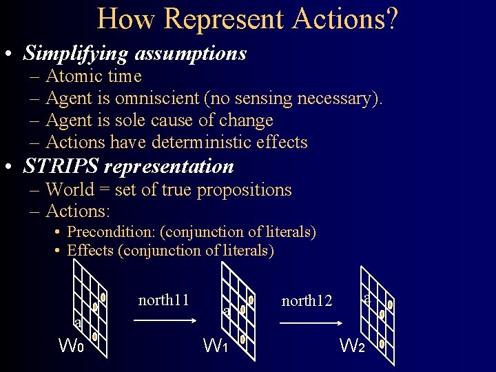
How Represent Actions? • Simplifying assumptions – Atomic time – Agent is omniscient (no sensing necessary). – Agent is sole cause of change – Actions have deterministic effects • STRIPS representation – World = set of true propositions – Actions: • Precondition: (conjunction of literals) • Effects (conjunction of literals) north 11 a W 0 a W 1 north 12 a W 2
Planning as Search • Nodes World states • Arcs Actions • Initial State The state satisfying the complete description of the initial conds • Goal State Any state satisfying the goal propositions
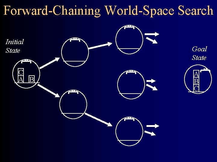
Forward-Chaining World-Space Search Initial State C A B Goal State A B C
Planning as Search 2 • Nodes Partially specified plans • Arcs Adding + deleting actions or constraints (e. g. <) to plan • Initial State The empty plan • Goal State A plan which when simulated achieves the goal
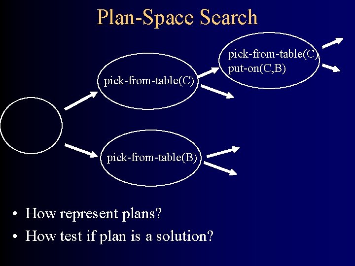
Plan-Space Search pick-from-table(C) pick-from-table(B) • How represent plans? • How test if plan is a solution? pick-from-table(C) put-on(C, B)
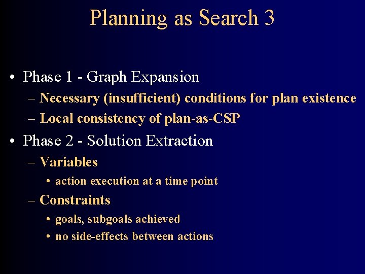
Planning as Search 3 • Phase 1 - Graph Expansion – Necessary (insufficient) conditions for plan existence – Local consistency of plan-as-CSP • Phase 2 - Solution Extraction – Variables • action execution at a time point – Constraints • goals, subgoals achieved • no side-effects between actions
Planning as Search 4 • Compile planning problem to propositional satisfiability - generate a set of clauses to satisfy. • Use a fast solver like GSAT or an incremental solver like an LTMS
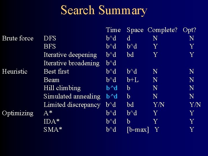
Search Summary Brute force Heuristic Optimizing Time DFS b^d BFS b^d Iterative deepening b^d Iterative broadening b^d Best first b^d Beam b^d Hill climbing b^d Simulated annealing b^d Limited discrepancy b^d A* b^d IDA* b^d SMA* b^d Space Complete? Opt? d N N b^d Y Y b^d b+L b b bd b^d b [b-max] N N N N Y/N Y Y Y
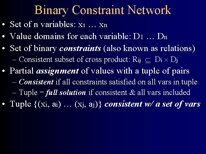
Binary Constraint Network • Set of n variables: x 1 … xn • Value domains for each variable: D 1 … Dn • Set of binary constraints (also known as relations) – Consistent subset of cross product: Rij Di Dj • Partial assignment of values with a tuple of pairs – Consistent if all constraints satisfied on all vars in tuple – Tuple = full solution if consistent & all vars included • Tuple {(xi, ai) … (xj, aj)} consistent w/ a set of vars
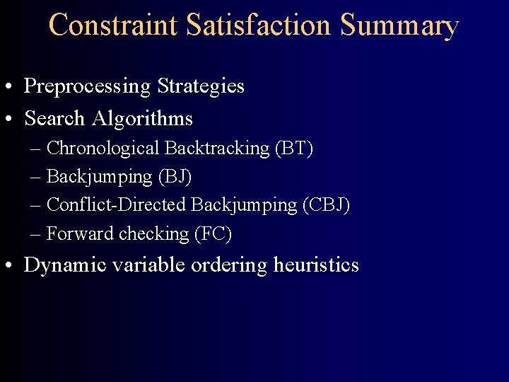
Constraint Satisfaction Summary • Preprocessing Strategies • Search Algorithms – Chronological Backtracking (BT) – Backjumping (BJ) – Conflict-Directed Backjumping (CBJ) – Forward checking (FC) • Dynamic variable ordering heuristics
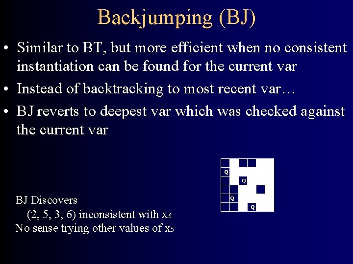
Backjumping (BJ) • Similar to BT, but more efficient when no consistent instantiation can be found for the current var • Instead of backtracking to most recent var… • BJ reverts to deepest var which was checked against the current var Q Q Q BJ Discovers (2, 5, 3, 6) inconsistent with x 6 No sense trying other values of x 5 Q Q

Other Strategies • CBJ – More sophisticated backjumping behavior – Each variable has conflict set CS • Set of vars that failed consistency checks w/ current val – Discovers (2, 5, 3) inconsistent with {x 5, x 6 } • FC – Perform Consistency Check Forward – Whenever assign var a value • Prune inconsistent values from • As-yet unvisited variables • Backtrack if domain of any var ever collapses
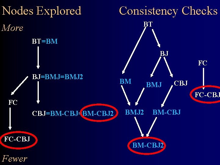
Nodes Explored Consistency Checks BT More BT=BM BJ FC BJ=BMJ 2 BM BMJ CBJ FC-CBJ FC CBJ=BM-CBJ 2 FC-CBJ Fewer BMJ 2 BM-CBJ 2
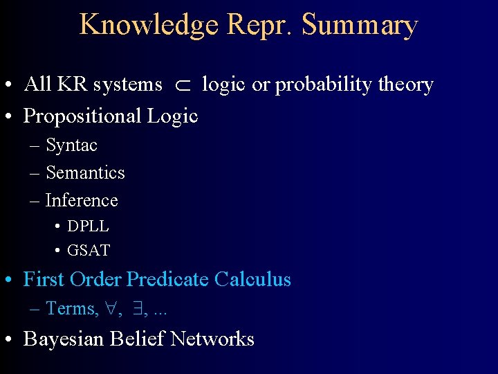
Knowledge Repr. Summary • All KR systems logic or probability theory • Propositional Logic – Syntac – Semantics – Inference • DPLL • GSAT • First Order Predicate Calculus – Terms, , , . . . • Bayesian Belief Networks
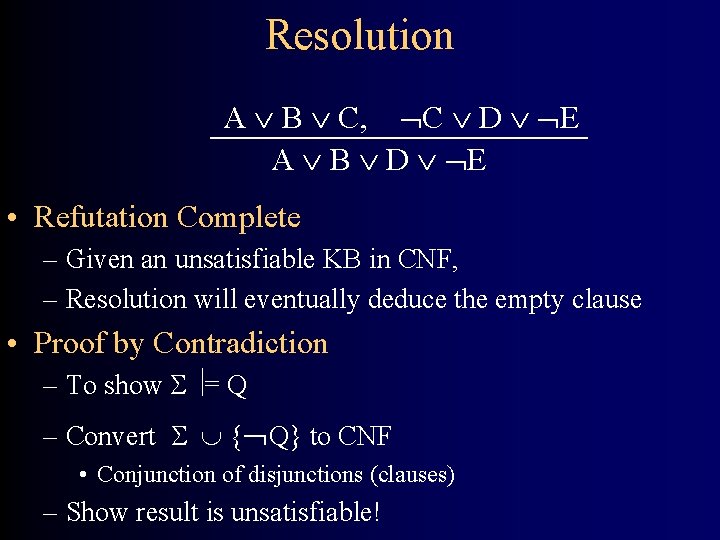
Resolution A B C, C D E A B D E • Refutation Complete – Given an unsatisfiable KB in CNF, – Resolution will eventually deduce the empty clause • Proof by Contradiction – To show = Q – Convert { Q} to CNF • Conjunction of disjunctions (clauses) – Show result is unsatisfiable!
![Davis Putnam (DPLL) [1962] Procedure DPLL (CNF formula: ) If is empty, return yes. Davis Putnam (DPLL) [1962] Procedure DPLL (CNF formula: ) If is empty, return yes.](http://slidetodoc.com/presentation_image_h2/a329075ecf3f1591ec3015b00305ebc8/image-63.jpg)
Davis Putnam (DPLL) [1962] Procedure DPLL (CNF formula: ) If is empty, return yes. If there is an empty clause in return no. If there is a pure literal u in return DPLL( (u)). If there is a unit clause {u} in return DPLL( (u)). Else Select a variable v mentioned in . If DPLL( (v))=yes, then return yes. Else return DPLL( ( v)). Recall: (u) means set u : = true in , then simplify
![GSAT [1992] Procedure GSAT (CNF formula: , max-restarts, max-climbs) For I : = I GSAT [1992] Procedure GSAT (CNF formula: , max-restarts, max-climbs) For I : = I](http://slidetodoc.com/presentation_image_h2/a329075ecf3f1591ec3015b00305ebc8/image-64.jpg)
GSAT [1992] Procedure GSAT (CNF formula: , max-restarts, max-climbs) For I : = I o max-restarts do A : = randomly generated truth assignment for j : = 1 to max-climbs do if A satisfies then return yes A : = random choice of one of best successors to A ; ; successor means only 1 var val changes from A ; ; best means making the most clauses true
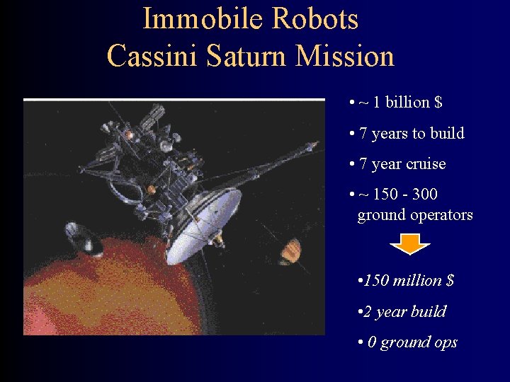
Immobile Robots Cassini Saturn Mission • ~ 1 billion $ • 7 years to build • 7 year cruise • ~ 150 - 300 ground operators • 150 million $ • 2 year build • 0 ground ops
Solution: Part 1 Model-based Programming Programmers and operators generate breadth of functions from commonsense hardware models in light of mission-level goals. Have engineers program in models, automate synthesis of code: – models are compositional & highly reusable. – generative approach covers broad set of behaviors. – commonsense models are easy to articulate at concept stage and insensitive to design variations.
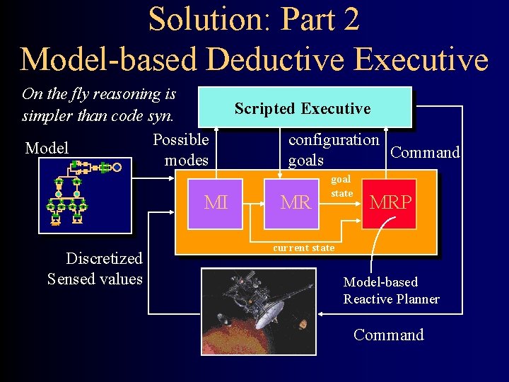
Solution: Part 2 Model-based Deductive Executive On the fly reasoning is simpler than code syn. Possible Model modes MI Discretized Sensed values Scripted Executive configuration Command goals MR goal state MRP current state Model-based Reactive Planner Command
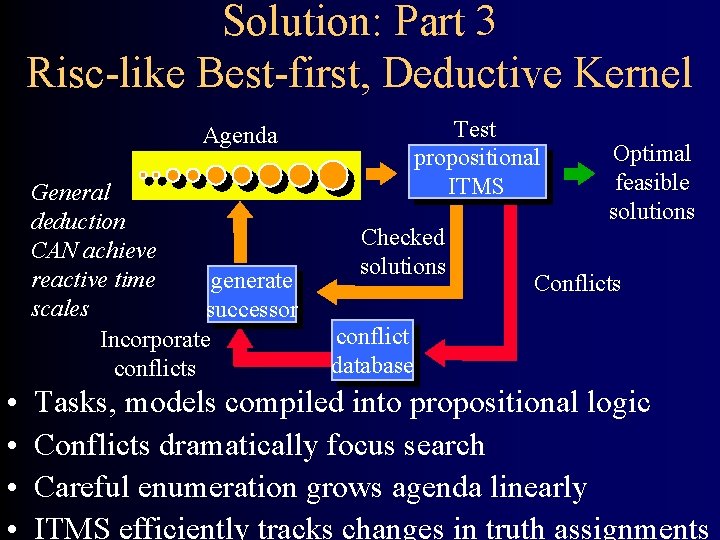
Solution: Part 3 Risc-like Best-first, Deductive Kernel Test propositional ITMS Agenda General deduction CAN achieve reactive time generate scales successor Incorporate conflicts • • Checked solutions Optimal feasible solutions Conflicts conflict database Tasks, models compiled into propositional logic Conflicts dramatically focus search Careful enumeration grows agenda linearly ITMS efficiently tracks changes in truth assignments
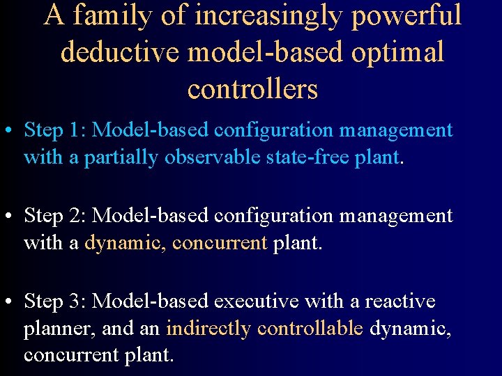
A family of increasingly powerful deductive model-based optimal controllers • Step 1: Model-based configuration management with a partially observable state-free plant. • Step 2: Model-based configuration management with a dynamic, concurrent plant. • Step 3: Model-based executive with a reactive planner, and an indirectly controllable dynamic, concurrent plant.
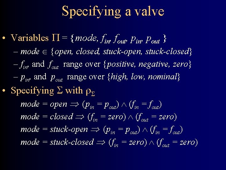
Specifying a valve • Variables = {mode, fin, fout, pin, pout } – mode {open, closed, stuck-open, stuck-closed} – fin, and fout range over {positive, negative, zero} – pin, and pout range over {high, low, nominal} • Specifying with mode = open (pin = pout) (fin = fout) mode = closed (fin = zero) (fout = zero) mode = stuck-open (pin = pout) (fin = fout) mode = stuck-closed (fin = zero) (fout = zero)
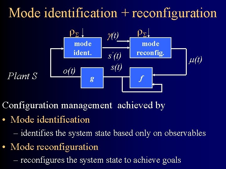
Mode identification + reconfiguration mode ident. Plant S o(t) g (t) s’(t) s(t) mode reconfig. (t) f Configuration management achieved by • Mode identification – identifies the system state based only on observables • Mode reconfiguration – reconfigures the system state to achieve goals
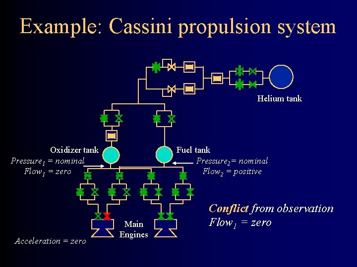
Example: Cassini propulsion system Helium tank Oxidizer tank Pressure 1 = nominal Flow 1 = zero Acceleration = zero Fuel tank Pressure 2= nominal Flow 2 = positive Main Engines Conflict from observation Flow 1 = zero
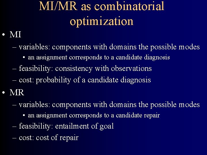
MI/MR as combinatorial optimization • MI – variables: components with domains the possible modes • an assignment corresponds to a candidate diagnosis – feasibility: consistency with observations – cost: probability of a candidate diagnosis • MR – variables: components with domains the possible modes • an assignment corresponds to a candidate repair – feasibility: entailment of goal – cost: cost of repair
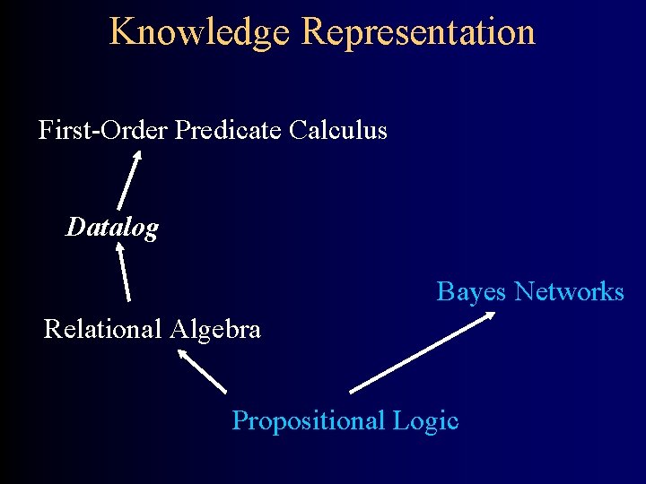
Knowledge Representation First-Order Predicate Calculus Datalog Bayes Networks Relational Algebra Propositional Logic
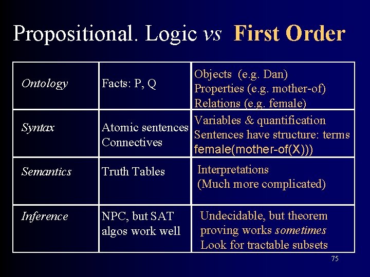
Propositional. Logic vs First Order Ontology Syntax Objects (e. g. Dan) Facts: P, Q Properties (e. g. mother-of) Relations (e. g. female) Variables & quantification Atomic sentences Sentences have structure: terms Connectives female(mother-of(X))) Semantics Truth Tables Interpretations (Much more complicated) Inference NPC, but SAT algos work well Undecidable, but theorem proving works sometimes Look for tractable subsets 75
![IIIIIS Representation III [Rajaraman 95] • Information Source Functionality – Info Required? $ Binding IIIIIS Representation III [Rajaraman 95] • Information Source Functionality – Info Required? $ Binding](http://slidetodoc.com/presentation_image_h2/a329075ecf3f1591ec3015b00305ebc8/image-76.jpg)
IIIIIS Representation III [Rajaraman 95] • Information Source Functionality – Info Required? $ Binding Patterns – Info Returned? – Mapping to World Ontology Source may be incomplete: (not ) • For Example IMDBActor($Actor, M) actor-in(M, Part, Actor) Spot($M, Rev, Y) Sidewalk($C, M, Th) review-of(M, Rev) & year-of(M, Y) shows-in(M, C, Th)
Query Planning • Given – Data source definitions (e. g. in datalog) – Query (written in datalog) • Produce – Plan to gather information • I. e. either a conjunctive query – Equivalent to a join of several information sources • Or a recursive datalog program – Necessary to account for functional dependencies, – Binding pattern restrictions – Maximality
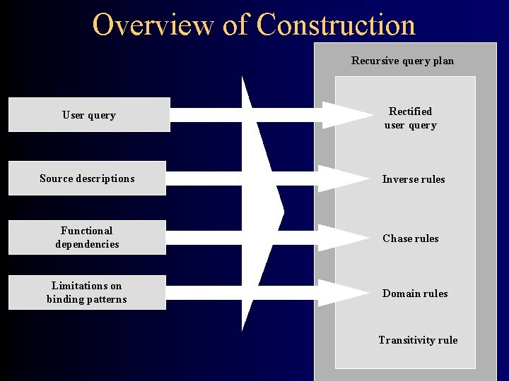
Overview of Construction Recursive query plan User query Rectified user query Source descriptions Inverse rules Functional dependencies Chase rules Limitations on binding patterns Domain rules Transitivity rule
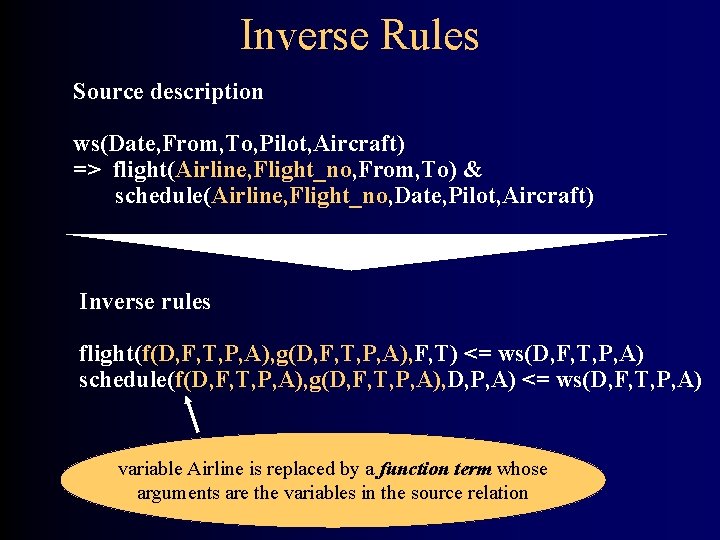
Inverse Rules Source description ws(Date, From, To, Pilot, Aircraft) => flight(Airline, Flight_no, From, To) & schedule(Airline, Flight_no, Date, Pilot, Aircraft) Inverse rules flight(f(D, F, T, P, A), g(D, F, T, P, A), F, T) <= ws(D, F, T, P, A) schedule(f(D, F, T, P, A), g(D, F, T, P, A), D, P, A) <= ws(D, F, T, P, A) variable Airline is replaced by a function term whose arguments are the variables in the source relation
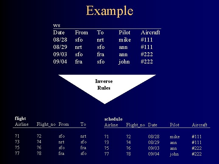
Example ws Date 08/28 08/29 09/03 09/04 From sfo nrt sfo fra To nrt sfo fra sfo Pilot mike ann john Aircraft #111 #222 Inverse Rules flight Airline Flight_no From ? 1 ? 3 ? 5 ? 7 ? 2 ? 4 ? 6 ? 8 sfo nrt sfo fra To schedule Airline Flight_no Date Pilot Aircraft nrt sfo fra sfo ? 1 ? 3 ? 5 ? 7 mike ann john #111 #222 ? 2 ? 4 ? 6 ? 8 08/29 09/03 09/04
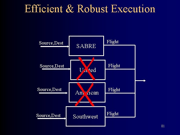
Efficient & Robust Execution Source, Dest SABRE United Flight Source, Dest American Flight Source, Dest Southwest Flight 81
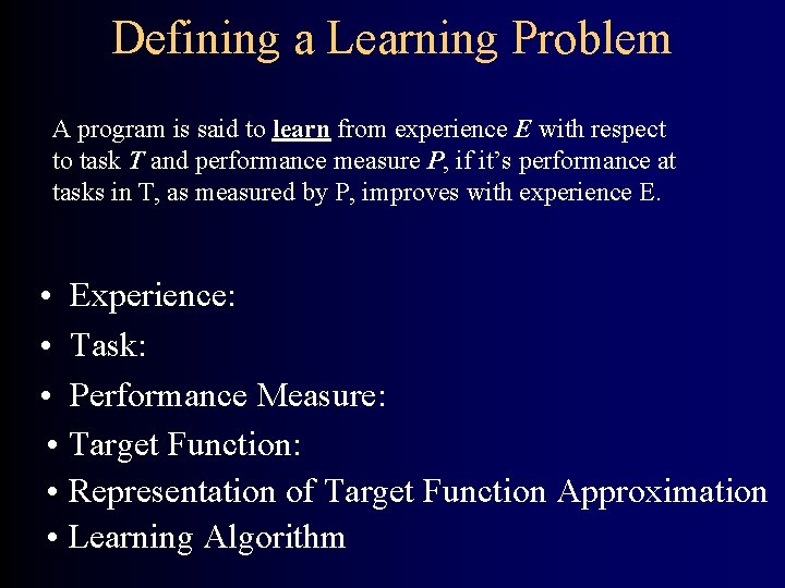
Defining a Learning Problem A program is said to learn from experience E with respect to task T and performance measure P, if it’s performance at tasks in T, as measured by P, improves with experience E. • Experience: • Task: • Performance Measure: • Target Function: • Representation of Target Function Approximation • Learning Algorithm
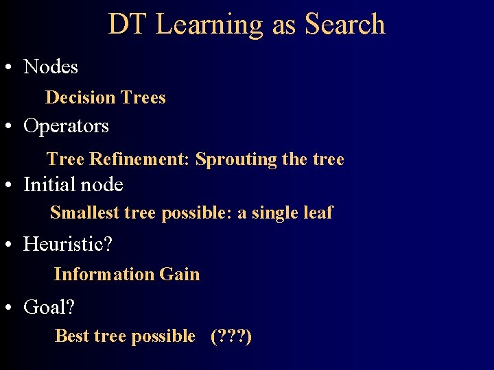
DT Learning as Search • Nodes Decision Trees • Operators Tree Refinement: Sprouting the tree • Initial node Smallest tree possible: a single leaf • Heuristic? Information Gain • Goal? Best tree possible (? ? ? )
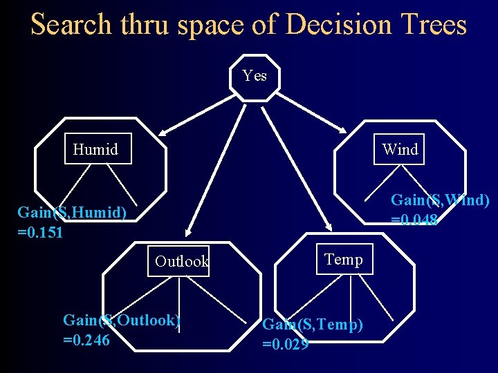
Search thru space of Decision Trees Yes Humid Wind Gain(S, Wind) =0. 048 Gain(S, Humid) =0. 151 Outlook Gain(S, Outlook) =0. 246 Temp Gain(S, Temp) =0. 029
![Resulting Tree …. Good day for tennis? Outlook Sunny No [2+, 3 -] Overcast Resulting Tree …. Good day for tennis? Outlook Sunny No [2+, 3 -] Overcast](http://slidetodoc.com/presentation_image_h2/a329075ecf3f1591ec3015b00305ebc8/image-85.jpg)
Resulting Tree …. Good day for tennis? Outlook Sunny No [2+, 3 -] Overcast Yes [4+] Now Recurse: Day Temp Humid Wind Tennis? d 1 h h weak n d 2 h h s n d 8 m h weak n d 9 c n weak yes d 11 m n s yes Rain No [2+, 3 -]
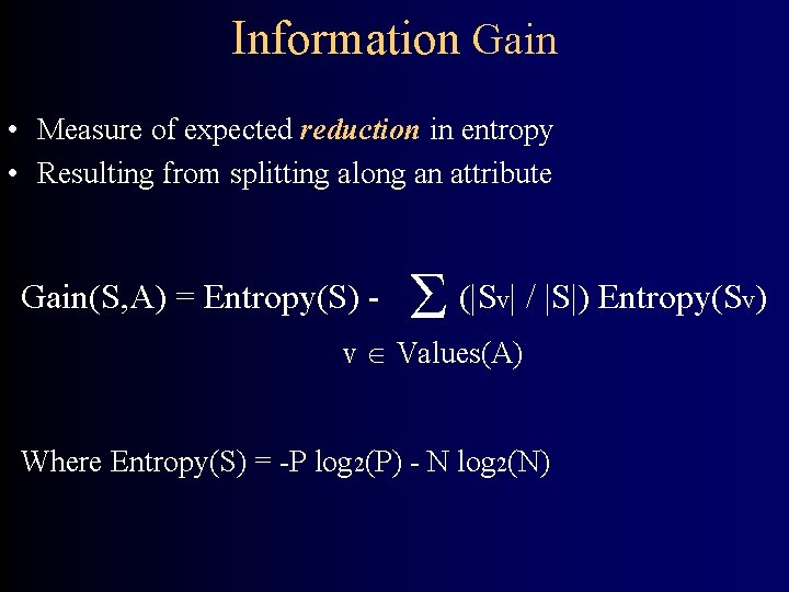
Information Gain • Measure of expected reduction in entropy • Resulting from splitting along an attribute Gain(S, A) = Entropy(S) - (|S | / |S|) Entropy(S ) v v Values(A) Where Entropy(S) = -P log 2(P) - N log 2(N) v
Overfitting… • DT is overfit when exists another DT’ and – DT has smaller error on training examples, but – DT has bigger error on test examples • Causes of overfitting – Noisy data, or – Training set is too small • Approaches – Stop before perfect tree, or – Postpruning
Comparison • Decision Tree learner searches a complete hypothesis space (one capable of representing any possible concept), but it uses an incomplete search method (hill climbing) • Candidate Elimination searches an incomplete hypothesis space (one capable of representing only a subset of the possible concepts), but it does so completely. Note: DT learner works better in practice
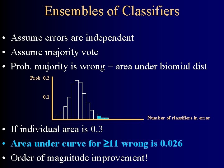
Ensembles of Classifiers • Assume errors are independent • Assume majority vote • Prob. majority is wrong = area under biomial dist Prob 0. 2 0. 1 Number of classifiers in error • If individual area is 0. 3 • Area under curve for 11 wrong is 0. 026 • Order of magnitude improvement!
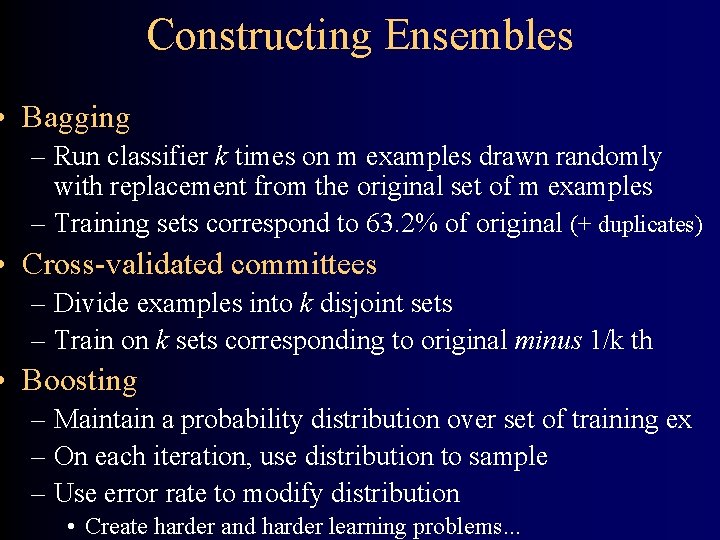
Constructing Ensembles • Bagging – Run classifier k times on m examples drawn randomly with replacement from the original set of m examples – Training sets correspond to 63. 2% of original (+ duplicates) • Cross-validated committees – Divide examples into k disjoint sets – Train on k sets corresponding to original minus 1/k th • Boosting – Maintain a probability distribution over set of training ex – On each iteration, use distribution to sample – Use error rate to modify distribution • Create harder and harder learning problems. . .
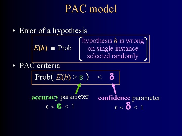
PAC model • Error of a hypothesis E(h) Prob hypothesis h is wrong on single instance selected randomly • PAC criteria Prob( E(h) > ) < accuracy parameter 0 < < 1 confidence parameter 0 < < 1
![Wrapper Induction [Kushmerick ‘ 97] machine learning techniques to automatically construct wrappers from examples Wrapper Induction [Kushmerick ‘ 97] machine learning techniques to automatically construct wrappers from examples](http://slidetodoc.com/presentation_image_h2/a329075ecf3f1591ec3015b00305ebc8/image-92.jpg)
Wrapper Induction [Kushmerick ‘ 97] machine learning techniques to automatically construct wrappers from examples <HTML><HEAD>Some Country Codes</HEAD> <BODY><B>Some Country Codes</B><P> <HTML><HEAD>Some Codes</HEAD> <B>Congo</B> <I>242</I><BR> <BODY><B>Some Country Codes</B><P> <HTML><HEAD>Some Codes</HEAD> <B>Egypt</B> <I>20</I><BR> <B>Congo</B> <I>242</I><BR> <BODY><B>Some Country Codes</B><P> <HTML><HEAD>Some Codes</HEAD> <B>Belize</B> <I>501</I><BR> <B>Egypt</B> <I>20</I><BR> <B>Congo</B> <I>242</I><BR> <BODY><B>Some Country Codes</B><P> <B>Spain</B> <I>34</I><BR> <B>Belize</B> <I>501</I><BR> <B>Egypt</B> <I>20</I><BR> <B>Congo</B> <I>242</I><BR> <HR><B>End</B></BODY></HTML> <B>Spain</B> <I>34</I><BR> <B>Belize</B> <I>501</I><BR> <B>Egypt</B> <I>20</I><BR> <HR><B>End</B></BODY></HTML> <B>Spain</B> <I>34</I><BR> <B>Belize</B> <I>501</I><BR> <HR><B>End</B></BODY></HTML> <B>Spain</B> <I>34</I><BR> <HR><B>End</B></BODY></HTML> wrapper procedure
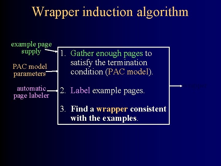
Wrapper induction algorithm example page supply PAC model parameters automatic page labeler 1. Gather enough pages to satisfy the termination condition (PAC model). 2. Label example pages. 3. Find a wrapper consistent with the examples. wrapper
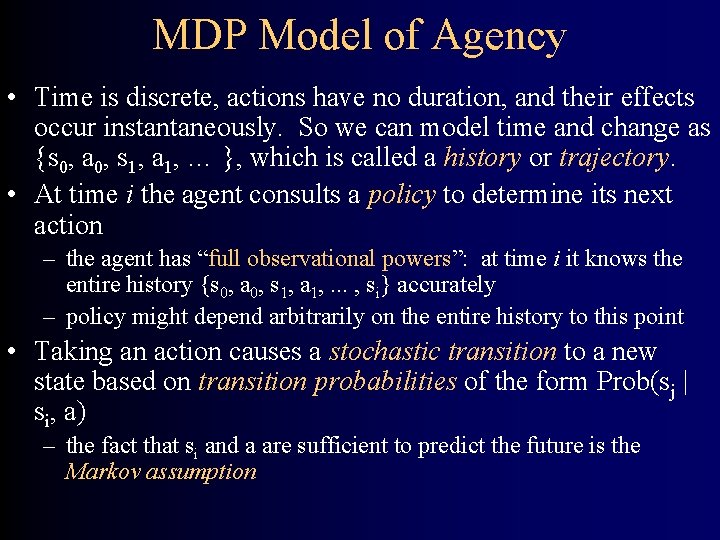
MDP Model of Agency • Time is discrete, actions have no duration, and their effects occur instantaneously. So we can model time and change as {s 0, a 0, s 1, a 1, … }, which is called a history or trajectory. • At time i the agent consults a policy to determine its next action – the agent has “full observational powers”: at time i it knows the entire history {s 0, a 0, s 1, a 1, . . . , si} accurately – policy might depend arbitrarily on the entire history to this point • Taking an action causes a stochastic transition to a new state based on transition probabilities of the form Prob(sj | si, a) – the fact that si and a are sufficient to predict the future is the Markov assumption
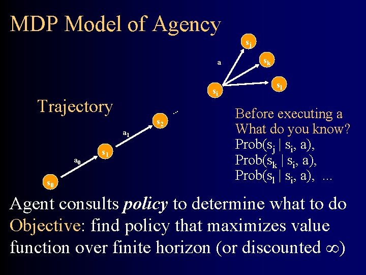
MDP Model of Agency sj a si Trajectory s 2 a 1 a 0 s 1 . . . sk sl Before executing a What do you know? Prob(sj | si, a), Prob(sk | si, a), Prob(sl | si, a), . . . Agent consults policy to determine what to do Objective: find policy that maximizes value function over finite horizon (or discounted )
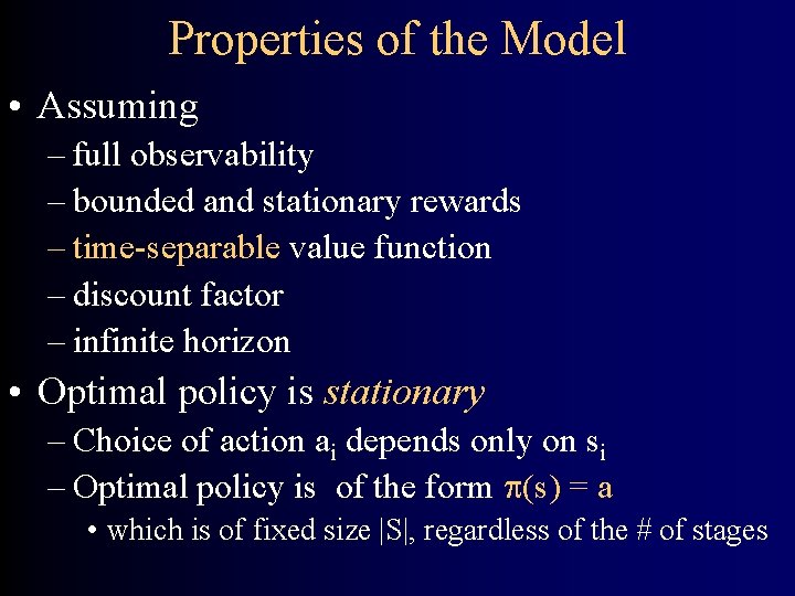
Properties of the Model • Assuming – full observability – bounded and stationary rewards – time-separable value function – discount factor – infinite horizon • Optimal policy is stationary – Choice of action ai depends only on si – Optimal policy is of the form (s) = a • which is of fixed size |S|, regardless of the # of stages
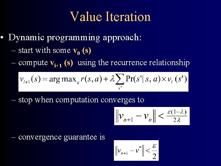
Value Iteration • Dynamic programming approach: – start with some v 0 (s) – compute vi+1 (s) using the recurrence relationship – stop when computation converges to – convergence guarantee is
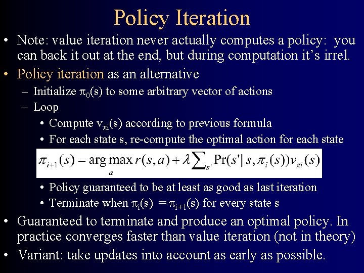
Policy Iteration • Note: value iteration never actually computes a policy: you can back it out at the end, but during computation it’s irrel. • Policy iteration as an alternative – Initialize 0(s) to some arbitrary vector of actions – Loop • Compute v i(s) according to previous formula • For each state s, re-compute the optimal action for each state • Policy guaranteed to be at least as good as last iteration • Terminate when i(s) = i+1(s) for every state s • Guaranteed to terminate and produce an optimal policy. In practice converges faster than value iteration (not in theory) • Variant: take updates into account as early as possible.
Reinforcement Learning • Avoid curse of modeling - Use experience instead! • Given only observed state and reward information, • Learn: – Transition probabilities – Reward function and discount factor – Optimal policy • Two main approaches: – learn the model then infer the policy – learn the policy without learning the explicit model parameters

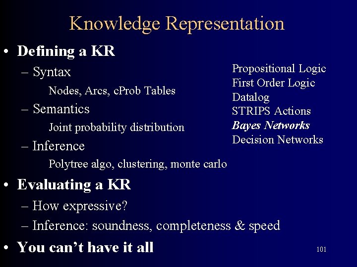
Knowledge Representation • Defining a KR – Syntax Nodes, Arcs, c. Prob Tables – Semantics Joint probability distribution – Inference Propositional Logic First Order Logic Datalog STRIPS Actions Bayes Networks Decision Networks Polytree algo, clustering, monte carlo • Evaluating a KR – How expressive? – Inference: soundness, completeness & speed • You can’t have it all 101

Basics • Random variable takes values – Cavity: yes or no Ache #Ache Cavity 0. 04 #Cavity 0. 01 0. 06 0. 89 • Joint Probability Distribution • Unconditional probability (“prior probability”) – P(A) – P(Cavity) = 0. 1 • Conditional Probability – P(A|B) – P(Cavity | Toothache) = 0. 8 • Bayes Rule – P(B|A) = P(A|B)P(B) / P(A) 102
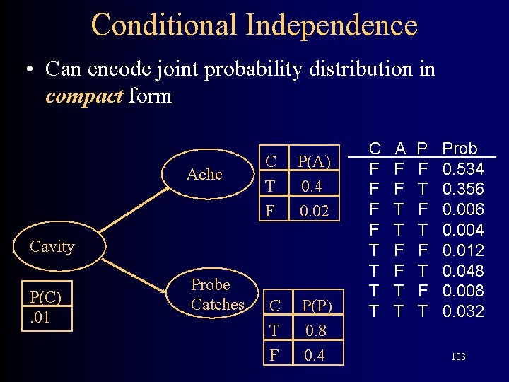
Conditional Independence • Can encode joint probability distribution in compact form Ache C T F P(A) 0. 4 0. 02 C T F P(P) 0. 8 0. 4 Cavity P(C). 01 Probe Catches C F F T T A F F T T P F T F T Prob 0. 534 0. 356 0. 004 0. 012 0. 048 0. 008 0. 032 103

Creating a Network • 1: Bayes net = representation of a JPD • 2: Bayes net = set of cond. independence statements • If create correct structure • Ie one representing causlity – Then get a good network • I. e. one that’s small = easy to compute with • One that is easy to fill in numbers 104
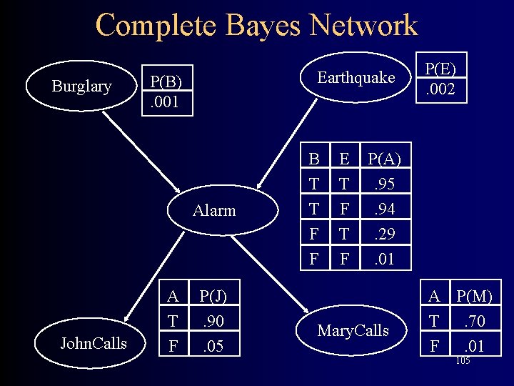
Complete Bayes Network Burglary Earthquake P(B). 001 Alarm John. Calls A T F P(J). 90. 05 B T T F F E T F P(E). 002 P(A). 95. 94. 29. 01 Mary. Calls A P(M) T. 70 F. 01 105
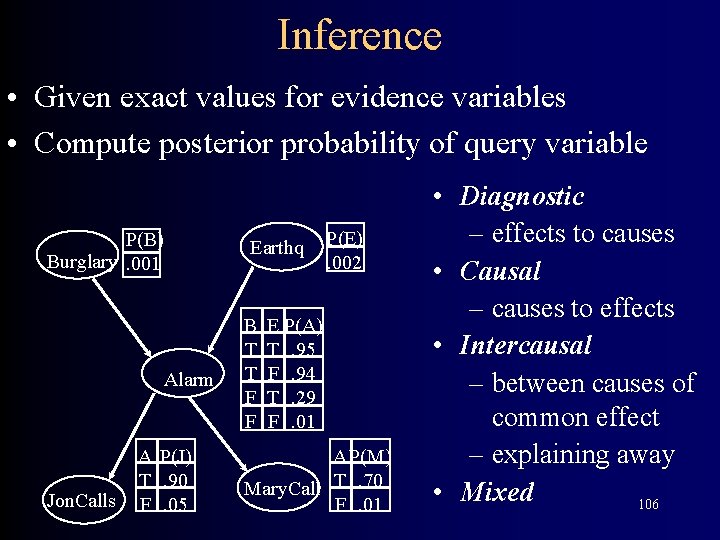
Inference • Given exact values for evidence variables • Compute posterior probability of query variable P(B) Burglary. 001 Alarm Jon. Calls A P(J) T. 90 F. 05 Earthq B T T F F P(E). 002 E P(A) T. 95 F. 94 T. 29 F. 01 A P(M) Mary. Call T. 70 F. 01 • Diagnostic – effects to causes • Causal – causes to effects • Intercausal – between causes of common effect – explaining away • Mixed 106

Algorithm • In general: NP Complete • Easy for polytrees – I. e. only one undirected path between nodes • Express P(X|E) by – 1. Recursively passing support from ancestor down • “Causal support” – 2. Recursively calc contribution from descendants up • “Evidential support” • Speed: linear in the number of nodes (in polytree) 107

Course Topics by Week • • • Search & Constraint Satisfaction Knowledge Representation 1: Propositional Logic Autonomous Spacecraft 1: Configuration Mgmt Autonomous Spacecraft 2: Reactive Planning Information Integration 1: Knowledge Representation Information Integration 2: Planning • • Information Integration 3: Execution; Learning 1 Learn 2: Supervised Learning Learn 3: Wrapper Induction & Reinforcement Learn Bayes Nets: Representation & Inference
- Slides: 108