Outline l Least Squares Methods l Estimation Least
- Slides: 34

Outline l Least Squares Methods l Estimation: Least Squares l Interpretation of estimators l Properties of OLS estimators l Variance of Y, b, and a l Hypothesis Test of b and a l ANOVA table l Goodness-of-Fit and R 2 (c) 2007 IUPUI SPEA K 300 (4392)

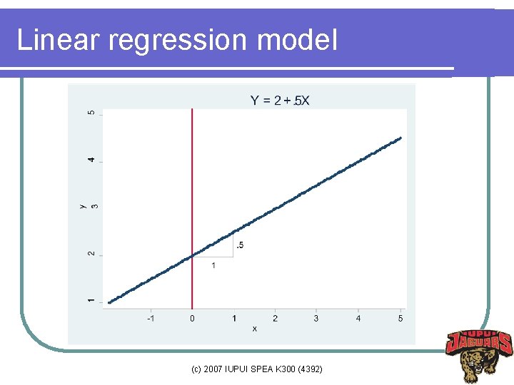
Linear regression model (c) 2007 IUPUI SPEA K 300 (4392)

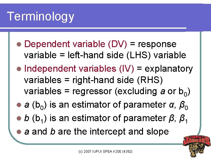
Terminology l Dependent variable (DV) = response variable = left-hand side (LHS) variable l Independent variables (IV) = explanatory variables = right-hand side (RHS) variables = regressor (excluding a or b 0) l a (b 0) is an estimator of parameter α, β 0 l b (b 1) is an estimator of parameter β, β 1 l a and b are the intercept and slope (c) 2007 IUPUI SPEA K 300 (4392)

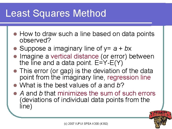
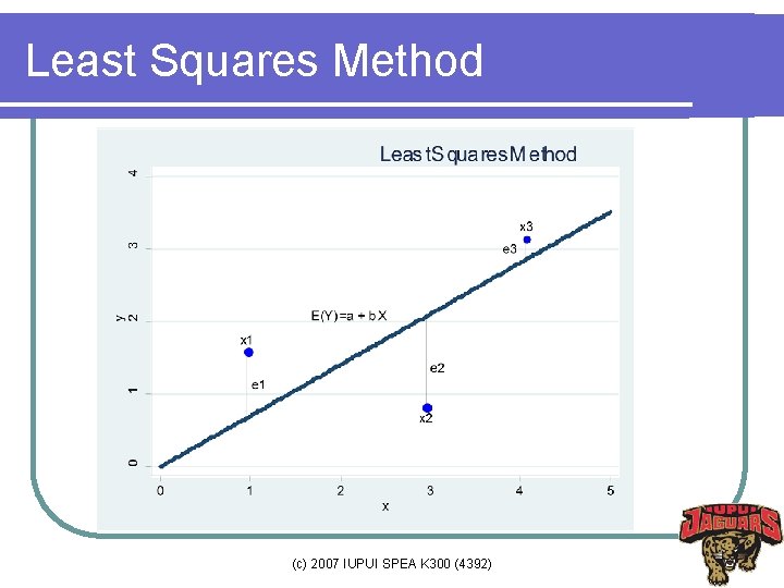
Least Squares Method l l l How to draw such a line based on data points observed? Suppose a imaginary line of y= a + bx Imagine a vertical distance (or error) between the line and a data point. E=Y-E(Y) This error (or gap) is the deviation of the data point from the imaginary line, regression line What is the best values of a and b? A and b that minimizes the sum of such errors (deviations of individual data points from the line) (c) 2007 IUPUI SPEA K 300 (4392)

Least Squares Method (c) 2007 IUPUI SPEA K 300 (4392)

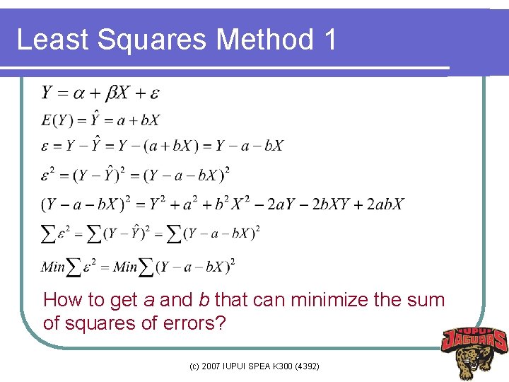
Least Squares Method l Deviation does not have good properties for computation l Why do we use squares of deviation? (e. g. , variance) l Let us get a and b that can minimize the sum of squared deviations rather than the sum of deviations. l This method is called least squares (c) 2007 IUPUI SPEA K 300 (4392)

Least Squares Method l l l Least squares method minimizes the sum of squares of errors (deviations of individual data points form the regression line) Such a and b are called least squares estimators (estimators of parameters α and β). The process of getting parameter estimators (e. g. , a and b) is called estimation “Regress Y on X” Lest squares method is the estimation method of ordinary least squares (OLS) (c) 2007 IUPUI SPEA K 300 (4392)

Ordinary Least Squares l Ordinary least squares (OLS) = l Linear regression model = l Classical linear regression model Linear relationship between Y and Xs l Constant slopes (coefficients of Xs) l Least squares method l Xs are fixed; Y is conditional on Xs l Error is not related to Xs l Constant variance of errors l (c) 2007 IUPUI SPEA K 300 (4392)

Least Squares Method 1 How to get a and b that can minimize the sum of squares of errors? (c) 2007 IUPUI SPEA K 300 (4392)

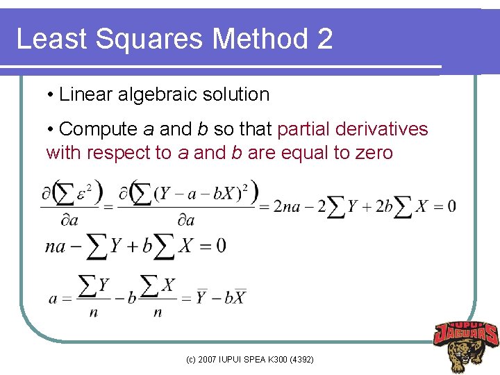
Least Squares Method 2 • Linear algebraic solution • Compute a and b so that partial derivatives with respect to a and b are equal to zero (c) 2007 IUPUI SPEA K 300 (4392)

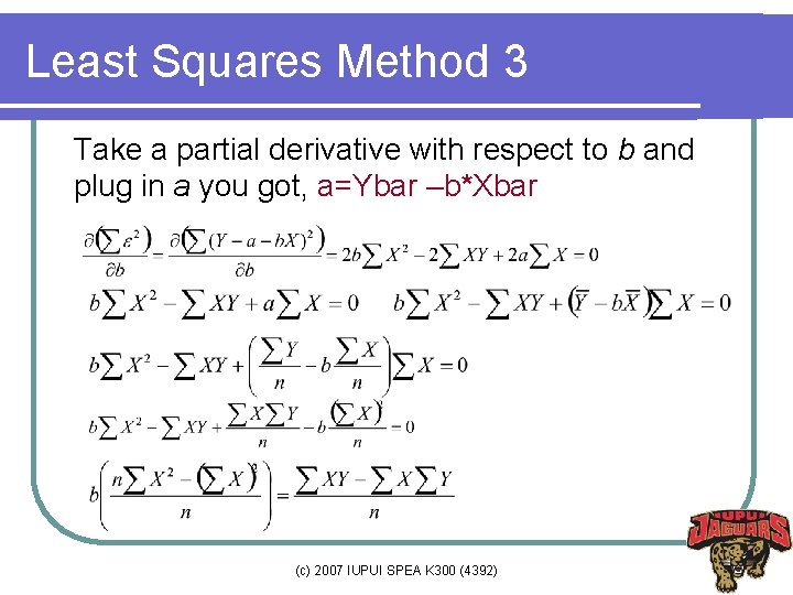
Least Squares Method 3 Take a partial derivative with respect to b and plug in a you got, a=Ybar –b*Xbar (c) 2007 IUPUI SPEA K 300 (4392)

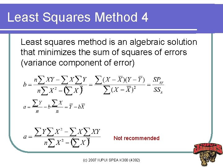
Least Squares Method 4 Least squares method is an algebraic solution that minimizes the sum of squares of errors (variance component of error) Not recommended (c) 2007 IUPUI SPEA K 300 (4392)

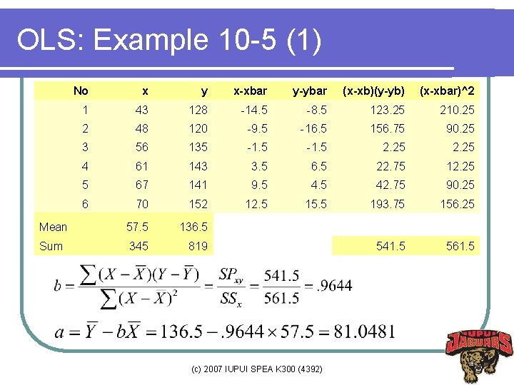
OLS: Example 10 -5 (1) No x y x-xbar y-ybar (x-xb)(y-yb) (x-xbar)^2 1 43 128 -14. 5 -8. 5 123. 25 210. 25 2 48 120 -9. 5 -16. 5 156. 75 90. 25 3 56 135 -1. 5 2. 25 4 61 143 3. 5 6. 5 22. 75 12. 25 5 67 141 9. 5 42. 75 90. 25 6 70 152 12. 5 15. 5 193. 75 156. 25 Mean 57. 5 136. 5 Sum 345 819 541. 5 561. 5 (c) 2007 IUPUI SPEA K 300 (4392)

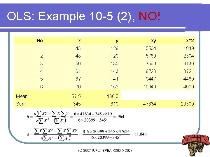
OLS: Example 10 -5 (2), NO! No x y xy x^2 1 43 128 5504 1849 2 48 120 5760 2304 3 56 135 7560 3136 4 61 143 8723 3721 5 67 141 9447 4489 6 70 152 10640 4900 Mean 57. 5 136. 5 Sum 345 819 47634 20399 (c) 2007 IUPUI SPEA K 300 (4392)

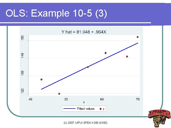
OLS: Example 10 -5 (3) (c) 2007 IUPUI SPEA K 300 (4392)

What Are a and b ? la is an estimator of its parameter α l a is the intercept, a point of y where the regression line meets the y axis l b is an estimator of its parameter β l b is the slope of the regression line l b is constant regardless of values of Xs l b is more important than a since that is what researchers want to know. (c) 2007 IUPUI SPEA K 300 (4392)

How to interpret b? l For unit increase in x, the expected change in y is b, holding other things (variables) constant. l For unit increase in x, we expect that y increases by. 964, holding other variables constant. (c) 2007 IUPUI SPEA K 300 (4392)

Properties of OLS estimators l l l The outcome of least squares method is OLS parameter estimators a and b. OLS estimators are linear OLS estimators are unbiased (precise) OLS estimators are efficient (small variance) Gauss-Markov Theorem: Among linear unbiased estimators, least square estimator (OLS estimator) has minimum variance. BLUE (best linear unbiased estimator) (c) 2007 IUPUI SPEA K 300 (4392)

Hypothesis Test of a an b l l l How reliable are a and b we compute? T-test (Wald test in general) can answer The standardized effect size (effect size / standard error) Effect size is a-0 and b-0 assuming 0 is the hypothesized value; H 0: α=0, H 0: β=0 Degrees of freedom is N-K, where K is the number of regressors +1 How to compute standard error (deviation)? (c) 2007 IUPUI SPEA K 300 (4392)

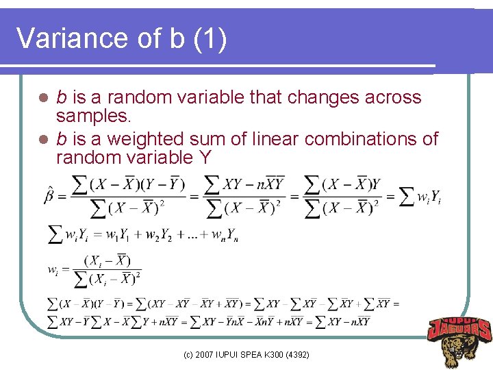
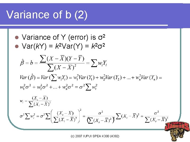
Variance of b (1) b is a random variable that changes across samples. l b is a weighted sum of linear combinations of random variable Y l (c) 2007 IUPUI SPEA K 300 (4392)

Variance of b (2) l l Variance of Y (error) is σ2 Var(k. Y) = k 2 Var(Y) = k 2σ2 (c) 2007 IUPUI SPEA K 300 (4392)

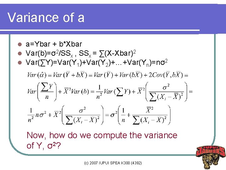
Variance of a l l l a=Ybar + b*Xbar Var(b)=σ2/SSx , SSx = ∑(X-Xbar)2 Var(∑Y)=Var(Y 1)+Var(Y 2)+…+Var(Yn)=nσ2 Now, how do we compute the variance of Y, σ2? (c) 2007 IUPUI SPEA K 300 (4392)

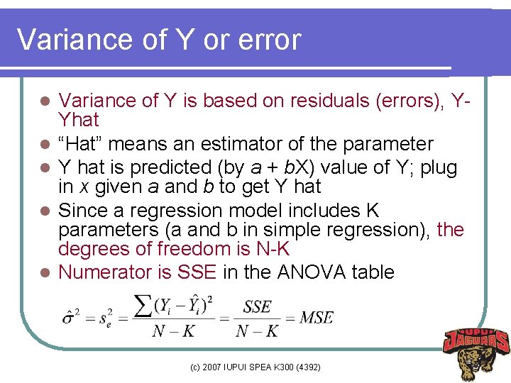
Variance of Y or error l l l Variance of Y is based on residuals (errors), YYhat “Hat” means an estimator of the parameter Y hat is predicted (by a + b. X) value of Y; plug in x given a and b to get Y hat Since a regression model includes K parameters (a and b in simple regression), the degrees of freedom is N-K Numerator is SSE in the ANOVA table (c) 2007 IUPUI SPEA K 300 (4392)

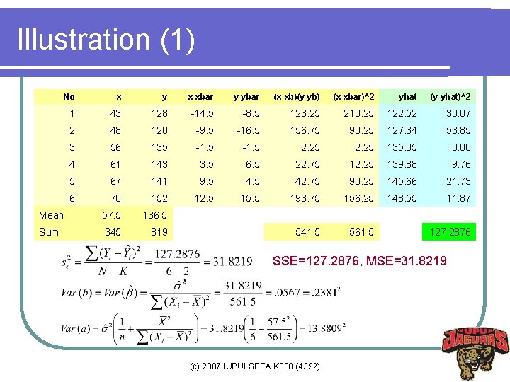
Illustration (1) No x y x-xbar y-ybar (x-xb)(y-yb) (x-xbar)^2 yhat (y-yhat)^2 1 43 128 -14. 5 -8. 5 123. 25 210. 25 122. 52 30. 07 2 48 120 -9. 5 -16. 5 156. 75 90. 25 127. 34 53. 85 3 56 135 -1. 5 2. 25 135. 05 0. 00 4 61 143 3. 5 6. 5 22. 75 12. 25 139. 88 9. 76 5 67 141 9. 5 42. 75 90. 25 145. 66 21. 73 6 70 152 12. 5 15. 5 193. 75 156. 25 148. 55 11. 87 Mean 57. 5 136. 5 Sum 345 819 541. 5 561. 5 127. 2876 SSE=127. 2876, MSE=31. 8219 (c) 2007 IUPUI SPEA K 300 (4392)

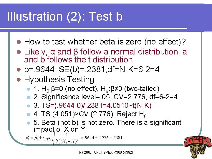
Illustration (2): Test b How to test whether beta is zero (no effect)? Like y, α and β follow a normal distribution; a and b follows the t distribution l b=. 9644, SE(b)=. 2381, df=N-K=6 -2=4 l Hypothesis Testing l l l l 1. H 0: β=0 (no effect), Ha: β≠ 0 (two-tailed) 2. Significance level=. 05, CV=2. 776, df=6 -2=4 3. TS=(. 9644 -0)/. 2381=4. 0510~t(N-K) 4. TS (4. 051)>CV (2. 776), Reject H 0 5. Beta (not b) is not zero. There is a significant impact of X on Y (c) 2007 IUPUI SPEA K 300 (4392)

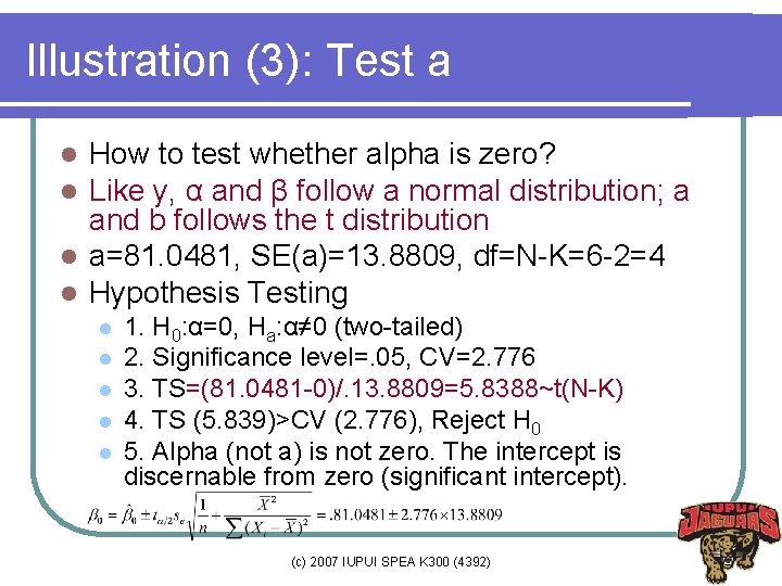
Illustration (3): Test a How to test whether alpha is zero? Like y, α and β follow a normal distribution; a and b follows the t distribution l a=81. 0481, SE(a)=13. 8809, df=N-K=6 -2=4 l Hypothesis Testing l l l l 1. H 0: α=0, Ha: α≠ 0 (two-tailed) 2. Significance level=. 05, CV=2. 776 3. TS=(81. 0481 -0)/. 13. 8809=5. 8388~t(N-K) 4. TS (5. 839)>CV (2. 776), Reject H 0 5. Alpha (not a) is not zero. The intercept is discernable from zero (significant intercept). (c) 2007 IUPUI SPEA K 300 (4392)

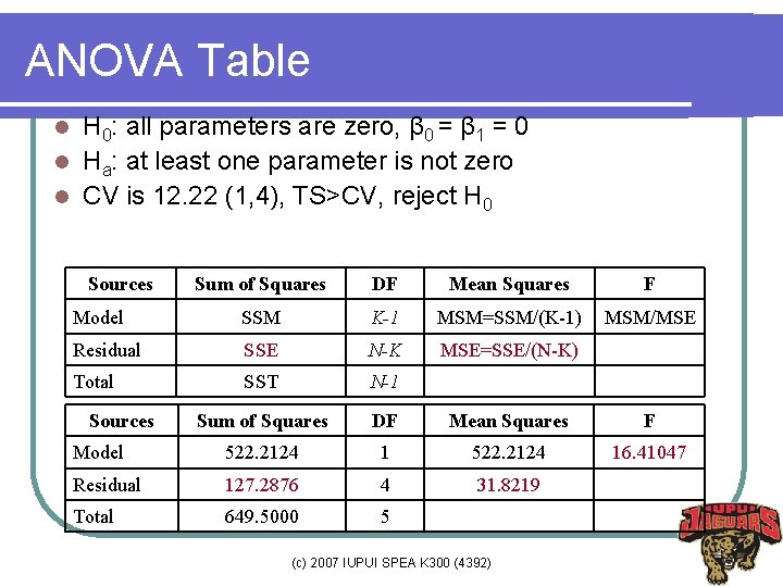
Questions l l l How do we test H 0: β 0(α)=β 1=β 2 …=0? Remember that t-test compares only two group means, while ANOVA compares more than two group means simultaneously. The same thing in linear regression. Construct the ANOVA table by partitioning variance of Y; F test examines the above H 0 The ANOVA table provides key information of a regression model (c) 2007 IUPUI SPEA K 300 (4392)

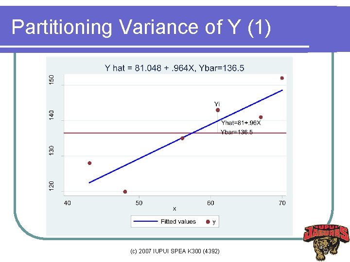
Partitioning Variance of Y (1) (c) 2007 IUPUI SPEA K 300 (4392)

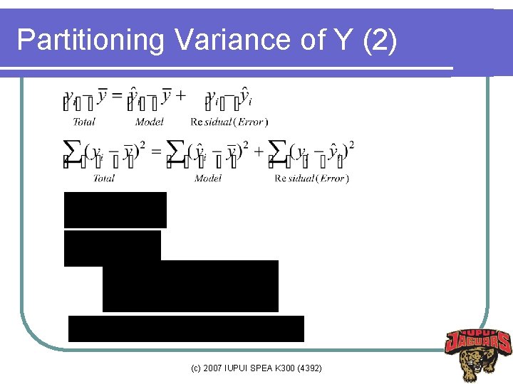
Partitioning Variance of Y (2) (c) 2007 IUPUI SPEA K 300 (4392)

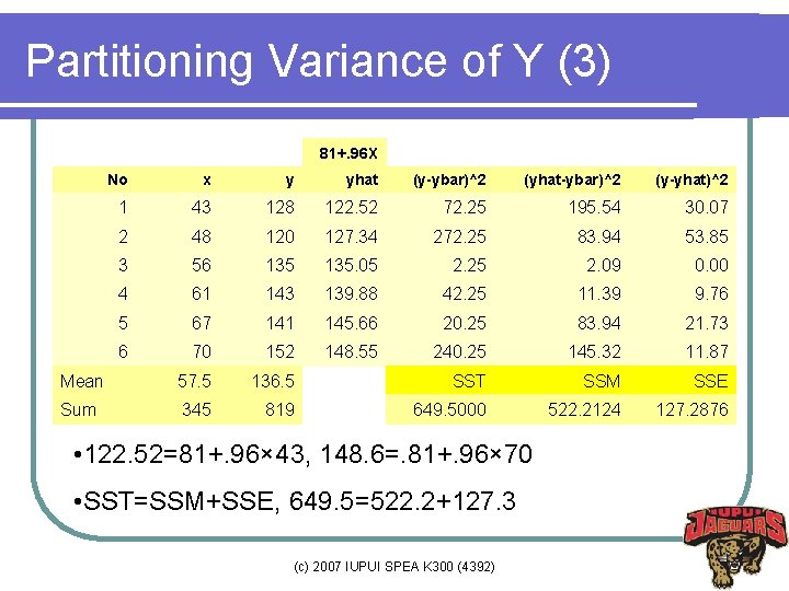
Partitioning Variance of Y (3) 81+. 96 X No x y yhat (y-ybar)^2 (yhat-ybar)^2 (y-yhat)^2 1 43 128 122. 52 72. 25 195. 54 30. 07 2 48 120 127. 34 272. 25 83. 94 53. 85 3 56 135. 05 2. 25 2. 09 0. 00 4 61 143 139. 88 42. 25 11. 39 9. 76 5 67 141 145. 66 20. 25 83. 94 21. 73 6 70 152 148. 55 240. 25 145. 32 11. 87 Mean 57. 5 136. 5 SST SSM SSE Sum 345 819 649. 5000 522. 2124 127. 2876 • 122. 52=81+. 96× 43, 148. 6=. 81+. 96× 70 • SST=SSM+SSE, 649. 5=522. 2+127. 3 (c) 2007 IUPUI SPEA K 300 (4392)

ANOVA Table H 0: all parameters are zero, β 0 = β 1 = 0 l Ha: at least one parameter is not zero l CV is 12. 22 (1, 4), TS>CV, reject H 0 l Sources Sum of Squares DF Mean Squares F Model SSM K-1 MSM=SSM/(K-1) MSM/MSE Residual SSE N-K MSE=SSE/(N-K) Total SST N-1 Sum of Squares DF Mean Squares F Model 522. 2124 16. 41047 Residual 127. 2876 4 31. 8219 Total 649. 5000 5 Sources (c) 2007 IUPUI SPEA K 300 (4392)

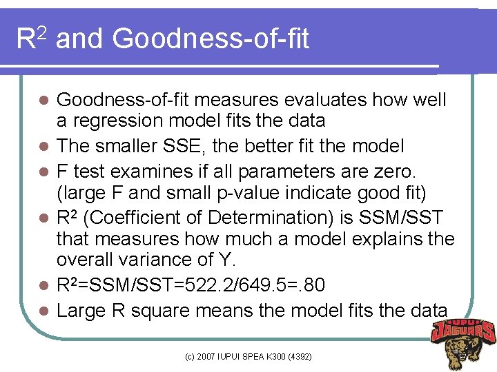
R 2 and Goodness-of-fit l l l Goodness-of-fit measures evaluates how well a regression model fits the data The smaller SSE, the better fit the model F test examines if all parameters are zero. (large F and small p-value indicate good fit) R 2 (Coefficient of Determination) is SSM/SST that measures how much a model explains the overall variance of Y. R 2=SSM/SST=522. 2/649. 5=. 80 Large R square means the model fits the data (c) 2007 IUPUI SPEA K 300 (4392)

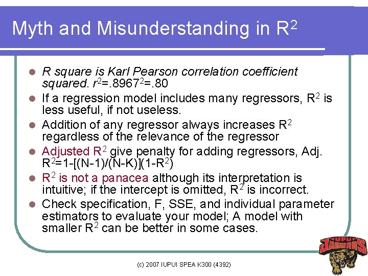
Myth and Misunderstanding in R 2 l l l R square is Karl Pearson correlation coefficient squared. r 2=. 89672=. 80 If a regression model includes many regressors, R 2 is less useful, if not useless. Addition of any regressor always increases R 2 regardless of the relevance of the regressor Adjusted R 2 give penalty for adding regressors, Adj. R 2=1 -[(N-1)/(N-K)](1 -R 2) R 2 is not a panacea although its interpretation is intuitive; if the intercept is omitted, R 2 is incorrect. Check specification, F, SSE, and individual parameter estimators to evaluate your model; A model with smaller R 2 can be better in some cases. (c) 2007 IUPUI SPEA K 300 (4392)

Interpolation and Extrapolation Confidence interval of E(Y|X), where x is within the rage of data x; interpolation l Confidence interval of Y|X, where x is beyond the range of data x; extrapolation l Extrapolation involves penalty and danger, which widens the confidence interval; less reliable l (c) 2007 IUPUI SPEA K 300 (4392)